Quantum Bootstrapping

Cassandra E. Granade
Centre for Engineered Quantum Systems

joint work with [Nathan Wiebe](http://research.microsoft.com/en-us/people/nawiebe/), Christopher Ferrie, and D. G. Cory [doi:10/tf3](https://dx.doi.org/10/tf3), [doi:10/tdk](https://dx.doi.org/10/tdk), and [doi:10/7nx](https://dx.doi.org/10/7nx) https://www.cgranade.com/research/talks/ipdf/10-2015/ $ \newcommand{\ee}{\mathrm{e}} \newcommand{\ii}{\mathrm{i}} \newcommand{\dd}{\mathrm{d}} \newcommand{\id}{𝟙} \newcommand{\TT}{\mathrm{T}} \newcommand{\defeq}{\mathrel{:=}} \newcommand{\Tr}{\operatorname{Tr}} \newcommand{\Var}{\operatorname{Var}} \newcommand{\Cov}{\operatorname{Cov}} \newcommand{\rank}{\operatorname{rank}} \newcommand{\expect}{\mathbb{E}} \newcommand{\sket}[1]{|#1\rangle\negthinspace\rangle} \newcommand{\sbraket}[1]{\langle\negthinspace\langle#1\rangle\negthinspace\rangle} \newcommand{\Gini}{\operatorname{Ginibre}} \newcommand{\supp}{\operatorname{supp}} \newcommand{\CC}{\mathbb{C}} $

Citations are listed by handle (e.g. 10/abc or 10012/abc) or arXiv number.
handle $\mapsto$ https://dx.doi.org/handle

We want to build a quantum computer.

As a prerequiste, we must be able to characterize the dynamics of large quantum systems, and to calibrate our control for these dynamics.

Formally, we need to learn the Hamiltonian $H$ of a system.

Our Strategy

- Express Hamiltonian learning in terms of simulation. - Substitute in quantum simulators.

Yields semiquantum algorithm that avoid classically-infeasible simulation calls.

We use physical insight to reduce the size of the quantum simulator needed.

Information locality provides a potentially-scalable characterization and calibration algorithm.

Bayesian Inference

Allows us to reduce learning to simulation.

$$ \Pr(\text{hypothesis} | \text{data}) = \frac{\Pr(\text{data} | \text{hypothesis})}{\Pr(\text{data})} \Pr(\text{hypothesis}) $$

- Prior $\Pr(\text{hypothesis})$ describes initial knowledge. - Posterior $\Pr(\text{hypothesis} | \text{data})$ describes what we learn from $\text{data}$. - Likelihood $\Pr(\text{data} | \text{hypothesis})$ represents simulation of experimental system.

Representing Hypotheses

We represent hypothetical Hamiltonians by a model $H = H(\vec{x})$ w/ params $\vec{x}$.

Example (Ising model): $ H(\vec{x}) = \sum_{i,j} x_{i,j} \sigma_z^{(i)} \sigma_z^{(j)}. $

$\mathrm{O}(n^2)$ parameters vs $\mathrm{O}(2^{2n})$ parameters.

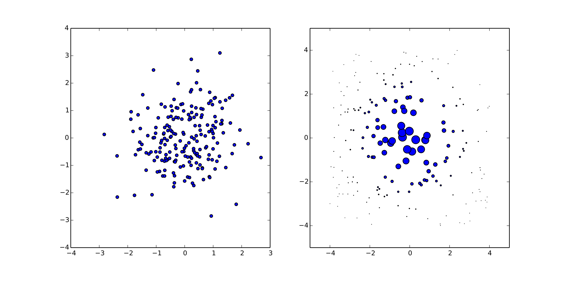
Sequential Monte Carlo

Represents distributions by finite sums for efficient numerical implementation.

\begin{align} \Pr(\vec{x}) & = \sum_{p \in \text{particles}} w_p \delta(\vec{x} - \vec{x}_p) \\ w_p & \mapsto w_p \times \Pr(\text{data} | \vec{x}_p) / \mathcal{N} \end{align}

Simulation is a resource to perform Bayes updates.

Liu-West Resampling (10/8c2) dynamically moves samples to recover numerical stability.

$\Pr(1 | \omega_1, \omega_2; t_1, t_2) = \cos^2(\omega_1 t_1 / 2) \cos^2(\omega_2 t_2 / 2)$

Already Useful!

- Classical Hamiltonian learning: [Granade *et al.* 10/s87](https://dx.doi.org/10/s87), [Stenberg *et al.* 10/7nw](https://dx.doi.org/10/7nw) - Randomized benchmarking: [Granade *et al.* 10/zmz](https://dx.doi.org/10/zmz) - Tomography: [Huszár and Houlsby 10/s86](https://dx.doi.org/10/s86), [Ferrie 10/7nt](https://dx.doi.org/10/7nt), [Granade *et al.* 1509.03770](https://scirate.com/arxiv/1509.03770)

More Than Just Learning

- Region estimation: [Granade *et al.* 10/s87](https://dx.doi.org/10/s87), [Ferrie 10/tb4](https://dx.doi.org/10/tb4) - Time-dependence (drift/diffusion): [Granade *et al.* 1509.03770](https://scirate.com/arxiv/1509.03770), [Granade 10012/9217](https://dx.doi.org/10012/9217), [Wiebe and Granade 1508.00869](https://scirate.com/arxiv/1508.00869)

Near-Optimal Performance for $H = \omega \sigma_z / 2$

QInfer

Extensible and flexible open-source library for Python.

Easy to Use


import qinfer as qi
model = qi.BinomialModel(qi.SimplePrecessionModel())
prior = qi.UniformDistribution([[0, 1]])
updater = qi.smc.SMCUpdater(model, 1200, prior)

Enough classical, though, let's get back to

Quantum Hamiltonian Learning.

Replace likelihood calls in the Bayes update with quantum likelihood evaluation, using trusted device.

Heuristics for experiment design are critical.

Particle Guess Heuristic

Draw $H_-$, $H_-'$ from posterior.
Evolve under $H_-$ for $t = 1 / \|H_- - H_-'\|$.

Simulation-free, uses current uncertainty to choose next experiment s.t. $t \|H_- - H\| \approx \text{const}$.

Scaling for Complete Ising Graph

QHL is Robust

We obtain accurate results even with sampling error, imperfect coupling, and approximate models.

Since QHL is robust to approximate models, use information locality (Lieb-Robinson bounds) to provide approximate compressed model.

Scan observable across trusted register and untrusted device.

Perform multiple rounds to reduce Lieb-Robinson velocity by current knowledge of $H$.

50-qubit untrusted device, 8-qubit simulator, 4-qubit observable

Calibrating for Crosstalk

Iterate compressed quantum Hamiltonian learning for each control Hamiltonian $H_i$.

\[ H(\vec{c}; \vec{x}) = H_0(\vec{x}) + \sum_i c_i H_i(\vec{x}) \]

- Characterizes the crosstalk, such that we can pre-compensate to get local control. --- - Pseudoinverse gives control settings to implement a bigger instance of quantum bootstrapping.

50-qubit untrusted device, 8-qubit simulator, 4-qubit observable, 300 measurements/scan

Conclusions

- Sequential Monte Carlo let us learn Hamiltonians with quantum resources. - Information locality enables using *smaller* trusted quantum resources. - Hamiltonian learning also learns crosstalk.

Quantum resources provide a path towards developing more powerful quantum resources.