Rejection and Particle Filtering for Hamiltonian Learning

Cassandra E. Granade
Centre for Engineered Quantum Systems $ \newcommand{\ee}{\mathrm{e}} \newcommand{\ii}{\mathrm{i}} \newcommand{\dd}{\mathrm{d}} \newcommand{\id}{𝟙} \newcommand{\TT}{\mathrm{T}} \newcommand{\defeq}{\mathrel{:=}} \newcommand{\Tr}{\operatorname{Tr}} \newcommand{\Var}{\operatorname{Var}} \newcommand{\Cov}{\operatorname{Cov}} \newcommand{\rank}{\operatorname{rank}} \newcommand{\expect}{\mathbb{E}} \newcommand{\sket}[1]{|#1\rangle\negthinspace\rangle} \newcommand{\sbraket}[1]{\langle\negthinspace\langle#1\rangle\negthinspace\rangle} \newcommand{\Gini}{\operatorname{Ginibre}} \newcommand{\supp}{\operatorname{supp}} \newcommand{\ket}[1]{\left|#1\right\rangle} \newcommand{\bra}[1]{\left\langle#1\right|} \newcommand{\braket}[1]{\left\langle#1\right\rangle} $

Learning Hamiltonians is critical to a range of QIP tasks:

Metrology: Learning magnetic fields, etc.
Calibration: Static field / pulse power / crosstalk, etc.
Debugging/Diagnosis: $T_2$ estimation, other noise finding
Verification/Validation: Analog and digital quantum simulation

### **Example**: Ramsey Estimation ### Suppose $H = \omega \sigma_z / 2$ for some unknown $\omega$. Traditional approach: - Prepare $\ket{+} \propto \ket{0} + \ket{1}$, measure “click” w/ pr.: $ \|\bra{+} \ee^{\ii \omega t \sigma_z / 2} \ket{+}\|^2 = \cos^2(\omega t / 2) $. - Repeat for many “shots” to estimate click pr. - Repeat for many times to estimate signal.

You'll get something that looks a bit like this:

What's $\omega$? Fourier transform and look at the peak.

We can do better. # $H = H(\vec{x})$. # Hamiltonian learning is a special case of *parameter estimation*: given data $D$, what is $\vec{x}$?

--- We want an approach that can work for small and large quantum devices alike.

To get there, we consider several different approaches to parameter estimation.

Analytic Sergeevich et al. c4vv95 Ferrie, Granade, and Cory tfx
Rejection filter Wiebe and Granade bk9d
Particle filter Doucet et al. bmch
Likelihood-free particle filter Ferrie and Granade tdj

### The Likelihood Function ### $\|\bra{+} \ee^{\ii \omega t \sigma_z / 2} \ket{+}\|^2$ defines probability $\Pr(d | \omega; t)$ for every outcome $d$, model $\omega$ and experiment $t$. Basis for both maximum-likelihood and Bayesian methods.

### Bayesian Parameter Estimation ### The likelihood tells us what we learn from data: $$ \Pr(\vec{x} | d; e) = \frac{\Pr(d | \vec{x}; e)}{\Pr(d | e)} \Pr(\vec{x}) $$ --- Estimate $\hat{x} = \expect[\vec{x} | d; e] = \int \vec{x} \Pr(\vec{x} | d; e)\dd \vec{x}$. - **Optimal** for mean—squared error.

Each posterior $\Pr(\vec{x} | d; e)$ encodes our uncertainty about $x$. What should we expect squared-error to be? **Scalar case**: $ \expect[(x - \hat{x})^2 | d; e] = \mathbb{V}[x \mid d; e]. $ **Vector case**: $\expect[(\vec{x} - \hat{x}) (\vec{x} - \hat{x})^\TT | d; e] = \Cov(\vec{x} | d; e)$.

We can use our posteriors to make *adaptive* decisions: $$ e_* = \operatorname{arg min}_e \expect_d[\mathbb{V}(x | d; e)] $$

### **Example**: $x = (\omega)$ ### Can analytically find posterior for Gaussian priors, use to adaptively choose $t_k$. ![](./figures/how-t2.png)

**Problem**: may be intractable to analytically compute $$ \hat{x} \defeq \int \Pr(\vec{x} | d; e) \dd\vec{x} = \int \frac{ \Pr(d | \vec{x}; e) }{ \int \Pr(d | \vec{x}; e) \Pr(\vec{x}) \dd\vec{x} } \Pr(\vec{x}) \dd\vec{x}. $$

--- **Answer**: numerically approximate $\int f(\vec{x}) \Pr(\vec{x} | d)\dd\vec{x}$. *Efficient* to use Monte Carlo integration if we can sample from $\Pr(\vec{x})$.

## Rejection Sampling ## Given samples from $\Pr(\vec{x})$ and likelihood function $\Pr(d | \vec{x}; e)$, how do we sample from posterior for datum $d$? - Draw $\vec{x} \sim \Pr(\vec{x})$, accept $\vec{x}$ w/ $\Pr(d | \vec{x}; e)$. Accepted samples are distributed according to posterior.

Rejection Sampling Isn't Enough

Let $D = {d_1, \dots, d_k}$ be a set of data.

$$ \Pr(\text{accept} | \vec{x}) = \Pr(D | \vec{x}) = \prod_{d \in D} \Pr(d | \vec{x}) \overset{k \to \infty}{\longrightarrow} 0. $$

Example: Biased Coin $x = (p)$

$\Pr(H | p) = p$, $d \in \{H, T\}$.

$p \approx 0.5 \Longrightarrow \Pr(d_1, \dots, d_k | p) \approx 1 / 2^k$.

We will accept exponentially few samples!

### Gaussian Resampling ### For each datum $d$, use rejection sampling to approximate posterior moments: - $\bar{x} \gets \expect[\vec{x} | d]$. - $\Sigma \gets \operatorname{Cov}[\vec{x} | d] = \expect[\vec{x} \vec{x}^\TT | d] - \bar{x} \bar{x}^\TT$.

--- At the next iteration, draw prior samples from Gaussian with these moments: $$ \vec{x} \mid d \sim \mathcal{N}(\bar{x}, \Sigma) $$ Keeps $\Pr(\text{accept}) \approx \text{constant}$.

Can compute $\bar{x}$, $\Sigma$ from one sample at a time by accumulating

$$ x_{\Sigma} = \sum x \text{ and } x^2_{\Sigma} = \sum x^2. $$

\begin{align} \bar{x} & = x_{\Sigma} / n_{\text{accept}} \\ \Sigma & = x^2_{\Sigma} / n_{\text{accept}} - \bar{x}^2. \end{align}

Welford's algorithm: numerically-stable modification.

Rejection Filtering (RejF)

Input: Prior mean $\bar{x}$, prior covariance $\Sigma$, number of attempts $m$.

For each datum $d$ and experiment $e$:

$n, \bar{x}', M_2 \gets 0$ Initialize Welford.
While $n < m$:

Draw $\vec{x} \sim \mathcal{N}(\bar{x}, \Sigma)$. Sample f/ prior.
Accept $\vec{x}$ w/ $\Pr(d | \vec{x}; e)$.
If accepted, update $n$, $\bar{x}'$, $M_2$.

$\bar{x} \gets \bar{x}'$, $\Sigma \gets M_2 / (n - 1)$. Est. moments.

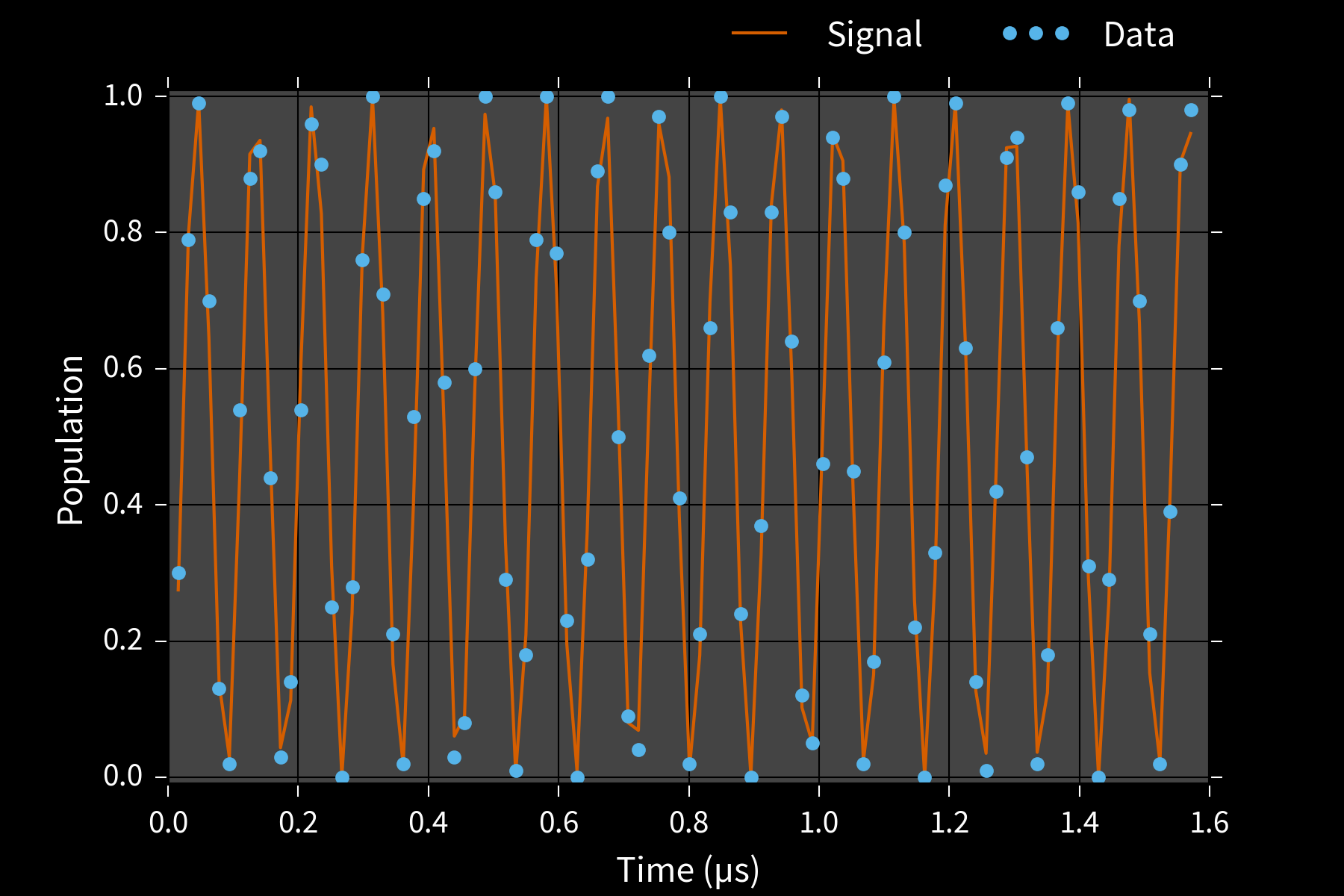
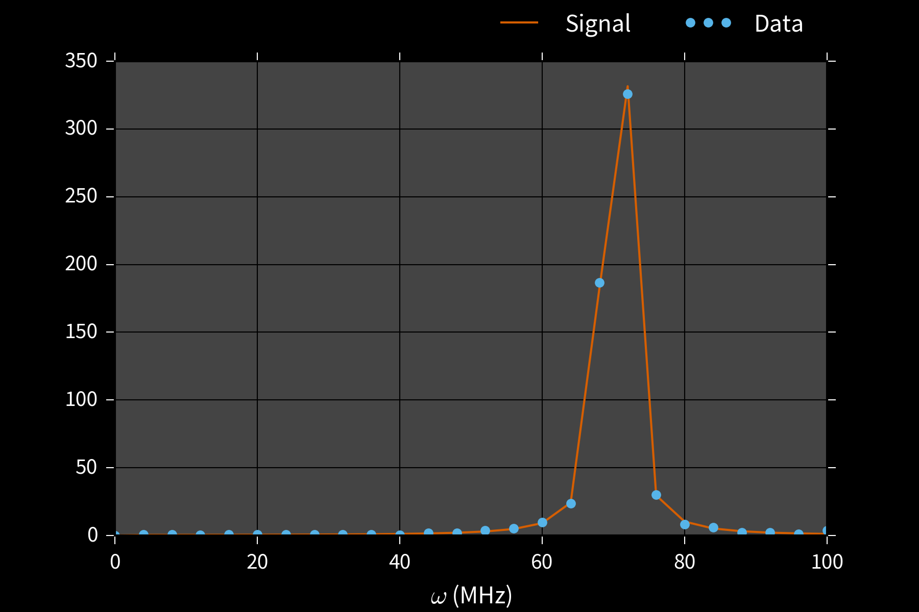
## Advantages of RejF ## - Accept pr based on a single datum ⇒ likelihood $\not\to 0$. - Easy to implement - Never needed to remember each accepted $x$! - Very low-memory (constant # of registers), ideal for FPGA use. - Easily parallelizable - “Reset rule” can abort from approximation failures.

Example: Phase Estimation, $x = (\phi)$

Prepare state $\ket{\phi}$ s. t. $U\ket{\phi} = \ee^{\ii \phi}\ket{\phi}$, measure to learn $\phi$.

$\theta = 0 \Rightarrow$ freq. est likelihood, w/ $\phi = \omega$, $M = t$.

Applications
Interferometry / metrology Higgins et al. crwd6w
Gate calibration / robust PE Kimmel et al. bmrg
Quantum simulation and chemistry Reiher et al. 1605.03590

Example: Phase Estimation, $x = (\phi)$

**Drawback**: RejF requires posterior after each datum to be $\approx$ Gaussian.

We can solve this by using a more general approach: - Weaken Gaussian assumption. - Generalize the rejection sampling step.

Liu-West Resampler

If we remember each sample $\vec{x}$, we can use them to relax RejF assumptions.

Input: $a, h \in [0, 1]$ s.t. $a^2 + h^2 = 1$, distribution $p(\vec{x})$.

Approximate $\bar{x} \gets \expect[\vec{x}]$, $\Sigma \gets \operatorname{Cov}(\vec{x})$
Draw parent $\vec{x}$ from $p(\vec{x})$.
Draw $\vec{\epsilon} \sim \mathcal{N}(0, \Sigma)$.
Return new sample $\vec{x}' \gets a \vec{x} + (1 - a) \bar{x} + h \vec{\epsilon}$.

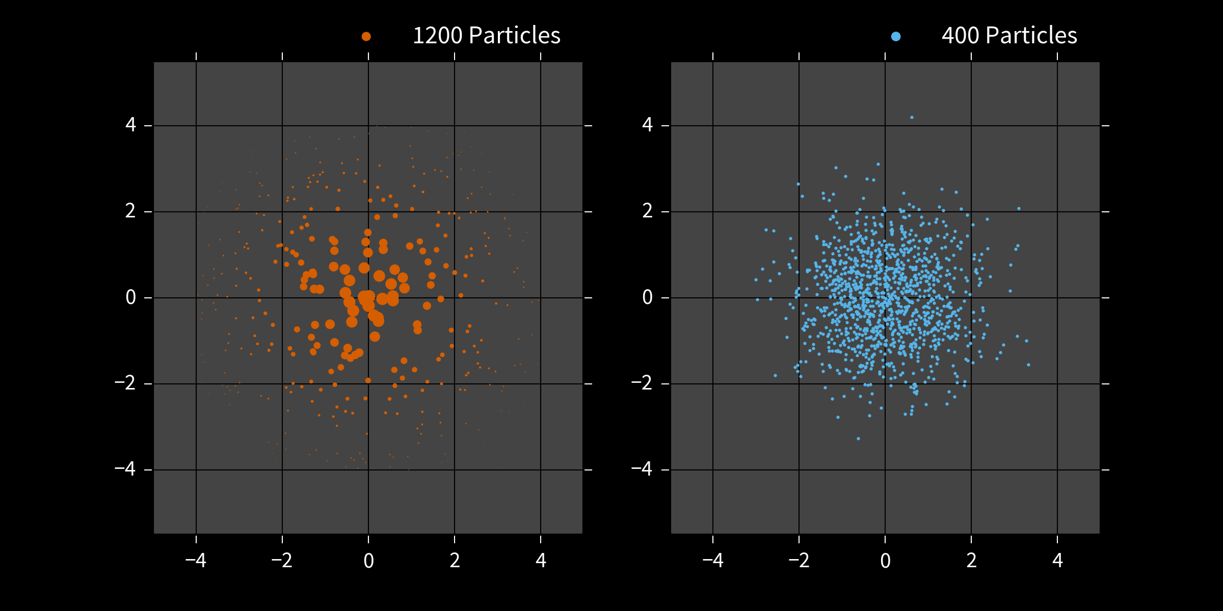
### Why Does Liu-West Work? ### \begin{align} \vec{x}' & \gets a \vec{x} + (1 - a) \bar{x} + h \vec{\epsilon} \\\\ \expect[\vec{x}'] & = [a + (1 - a)] \bar{x} \\\\ \Cov(\vec{x}') & = (a^2 + h^2) \Cov(\vec{x}). \\\\ \Longrightarrow a^2 + h^2 & = 1 \text{ preserves } \expect[\vec{x}], \Cov(\vec{x}). \end{align} --- Mixes original approximation with $1 - a$ of a Gaussian matching moments. - $a \to 0$: RejF (assumed density) approx - $a \to 1$: Bootstrap - $a = 0.98$: typical case (2% Gaussian).

### From Samples to Particles ### Define a particle $(w_i, \vec{x}_i)$ as a sample $\vec{x}_i$ and a weight $w_i \in [0, 1]$. - $\expect[\vec{x}] = \sum_i w_i \vec{x}_i$ - $\Cov(\vec{x}) = \sum_i w_i \vec{x}_i \vec{x}_i^\TT - \expect[\vec{x}]\expect^\TT[\vec{x}]$ - $\expect[f(\vec{x})] = \sum_i w_i f(\vec{x}_i)$ --- Corresponds to $ p(\vec{x}) \approx \sum_i w_i \delta(\vec{x} - \vec{x}_i). $

Particles can represent distributions using either
weights or positions.

Particle Filter

Draw $N$ initial samples $\vec{x}_i$ from the prior $\Pr(\vec{x})$ w/ uniform weights.
Instead of rej. sampling, update weights by \begin{align} \tilde{w}_i & = w_i \times \Pr(d | \vec{x}_i; e) \end{align}
Renormalize. \begin{align} w_i & \mapsto \tilde{w}_i / \sum_i \tilde{w}_i \end{align}
Periodically use Liu-West to draw new $\{\vec{x}_i\}$ with uniform weights. Store posterior in positions.

Useful for Hamiltonian models...

Rabi/Ramsey/Phase est. Granade et al. s87
Swap spectroscopy Stenberg et al. 7nw

...as well as other QIP tasks.

Tomography Huszár and Holsby s86 Struchalin et al. bmg5 Ferrie 7nt Granade et al. bhdw, 1605.05039
Randomized benchmarking Granade et al. zmz
Continuous measurement Chase and Geremia chk4q7
Interferometry/metrology Granade 10012/9217

### **Example**: $\vec{x} = (\omega, T_2)$ ### ![](figures/unknown-t2.png)

Example: $\vec{x} =$ COSY / Crosstalk

$ H(\omega_1, \omega_2, J) = \frac12 \left( \omega_1 \sigma_z \otimes \id + \omega_2 \id \otimes \sigma_z + J \sigma_z \otimes \sigma_z \right) $

Example: $\vec{x} =$ COSY / Crosstalk

Error Bars

Particle filters also yield credible regions $X_\alpha$ s.t. $$ \Pr(\vec{x} \in X_\alpha | d; e) \ge \alpha. $$

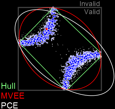
E.g.: Posterior covariance ellipse, convex hull, MVEE.

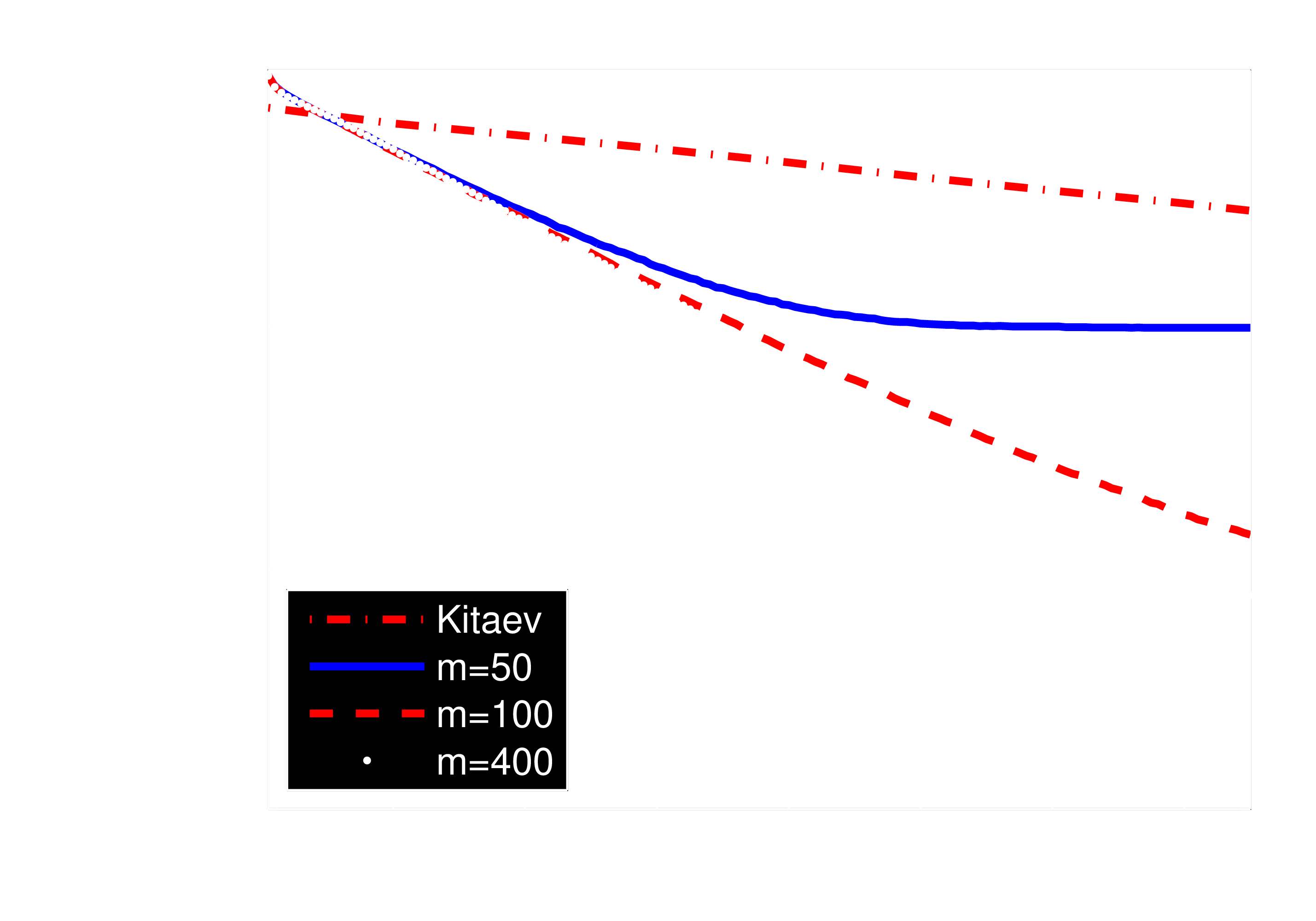
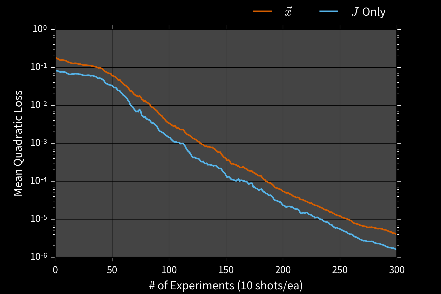
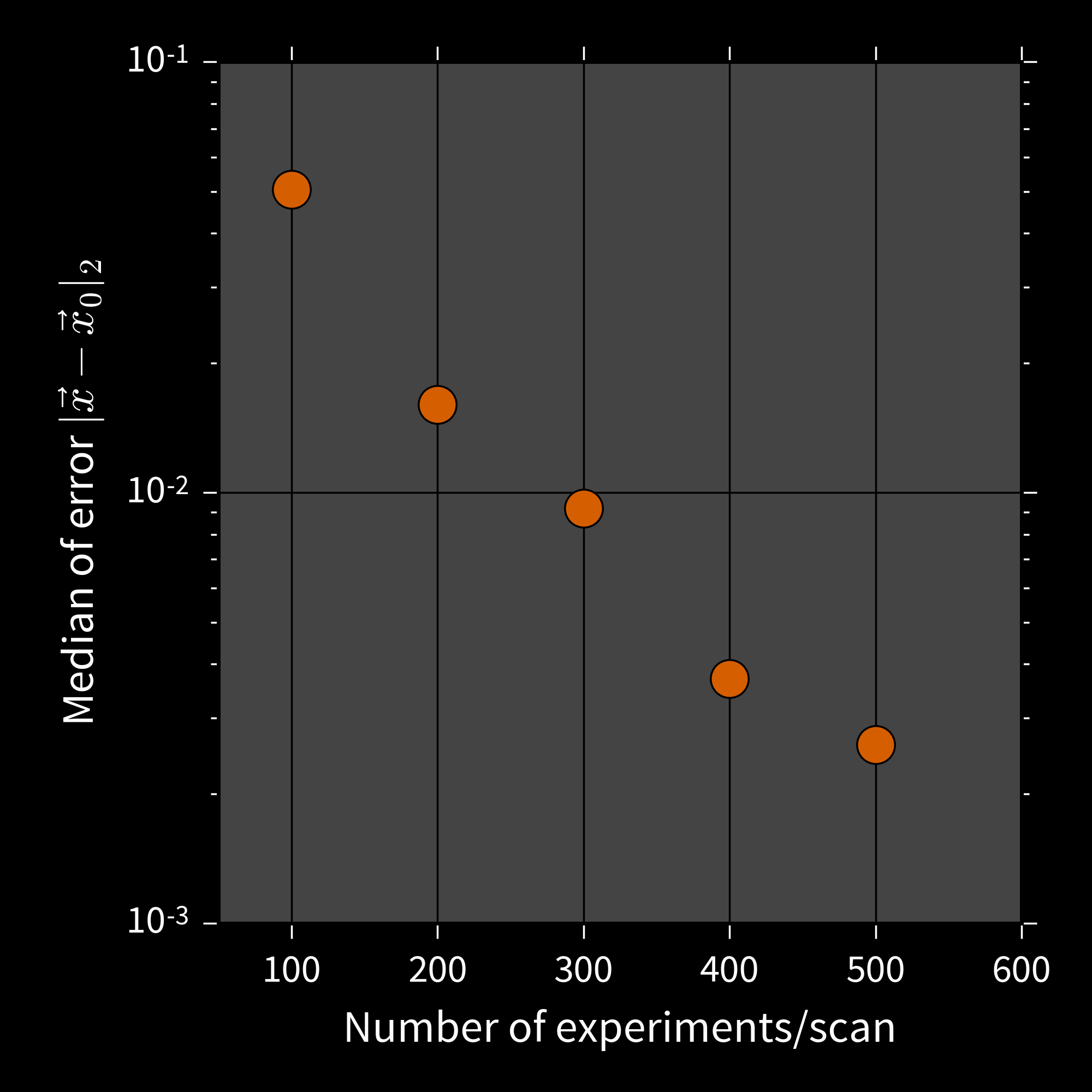
#### **QInfer**: Particle Filter Implementation for Quantum Info #### We provide an open-source implementation for use in experiment and theory alike. Written in Python, works with MATLAB and Julia.

Assessing Performance

Risk: average error given $\color{white}{\vec{x}}$
Bayes risk: average error over $\color{white}{\vec{x}}$

--- - Exact $\hat{x}$ optimal for Bayes risk / squared error. - Difficult to *prove* particle filter risk; find in special cases or by running many trials.

Simulation Costs

\begin{align} \tilde{w}_i & = w_i \times \color{red}{\Pr(d | \vec{x}_i; e)} \\ w_i & \mapsto \tilde{w}_i / \sum_i \tilde{w}_i \end{align}

- $\Pr(d | \vec{x}_i; e)$ is a *simulation*. - Need to simulate for each particle (~1000s calls/datum). - Infeasible for large quantum models. Let's do better: use *quantum* simulation instead.

### Two Kinds of Simulation ### ![](figures/simulators.png) Weak simulators produce *plausible datasets*.

### Likelihood-Free RejF ### Replace rej. sampling step by drawing datum from likelihood instead of computing exact value: - Draw datum $d'$ from $\Pr(d | \vec{x}; e)$. - Accept $\vec{x}$ if $d = d'$.

### Likelihood-Free Particle Filtering ### Can also use frequencies $f$ from weak simulation to approximate likelihoods in particle filtering. $$ \widehat{\Pr}(d | \vec{x}; e) = \frac{f(d | \vec{x}; e)}{k} $$ $k$: number of weak simulation calls used.

#### **Example**: Noisy Coin #### How well can we learn the bias $x = (p)$ of a noisy coin? $$ \Pr(\text{click} | p) = 0.95 p + 0.1 (1 - p) $$

### Quantum Hamiltonian Learning ### ![](figures/qle.png)

### **Example**: Nearest-Neighbor 1D Ising ### ![](figures/qle-line-ising.png)

We can do more with access to a *trusted* simulator. ### Quantum Interactivity ### ![](figures/iqle.png) Perform weak simulations on trusted device only.

We design experiments using the

PGH: Particle Guess Heuristic

Draw $\vec{x}_-, \vec{x}_-'$ from current posterior.
Let $t = 1 / |\vec{x}_- - \vec{x}_-'|$.
Return $e = (\vec{x}_-, t)$.

Adaptively chooses experiments such that
$t |\vec{x}_- - \vec{x}_-'| \approx\,$ constant.

### **Example**: Ising on Complete Graph ### ![](figures/iqle-complete-ising.png)

Robust even to wrong model. ($0.5$ NN + $10^{-4}$ Complete) ![](figures/qhl-bad-model.png)

One important approximation: physical locality.

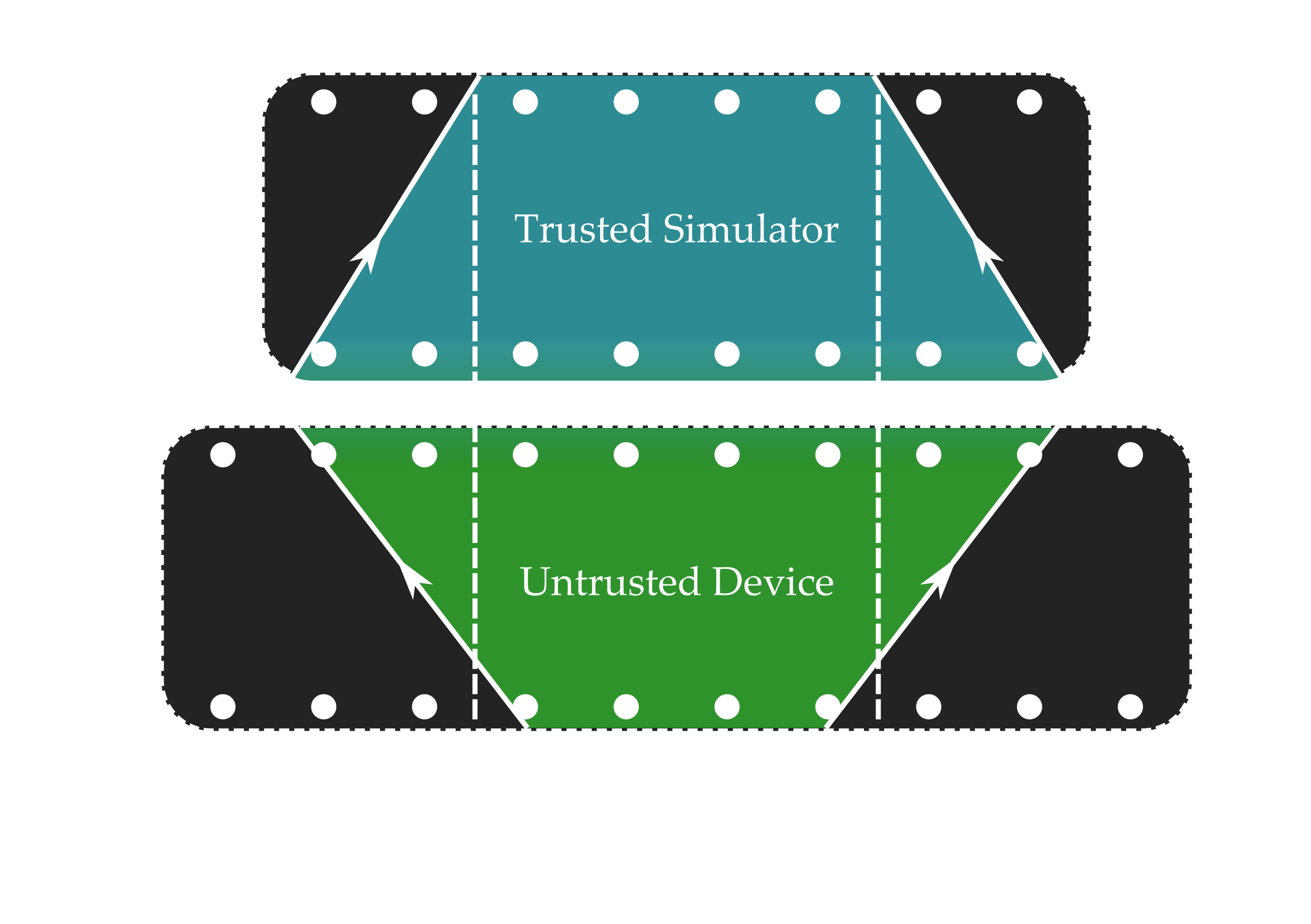
Approximation quality can be bounded if Lieb-Robinson velocity is finite.

Scan trusted device across untrusted.

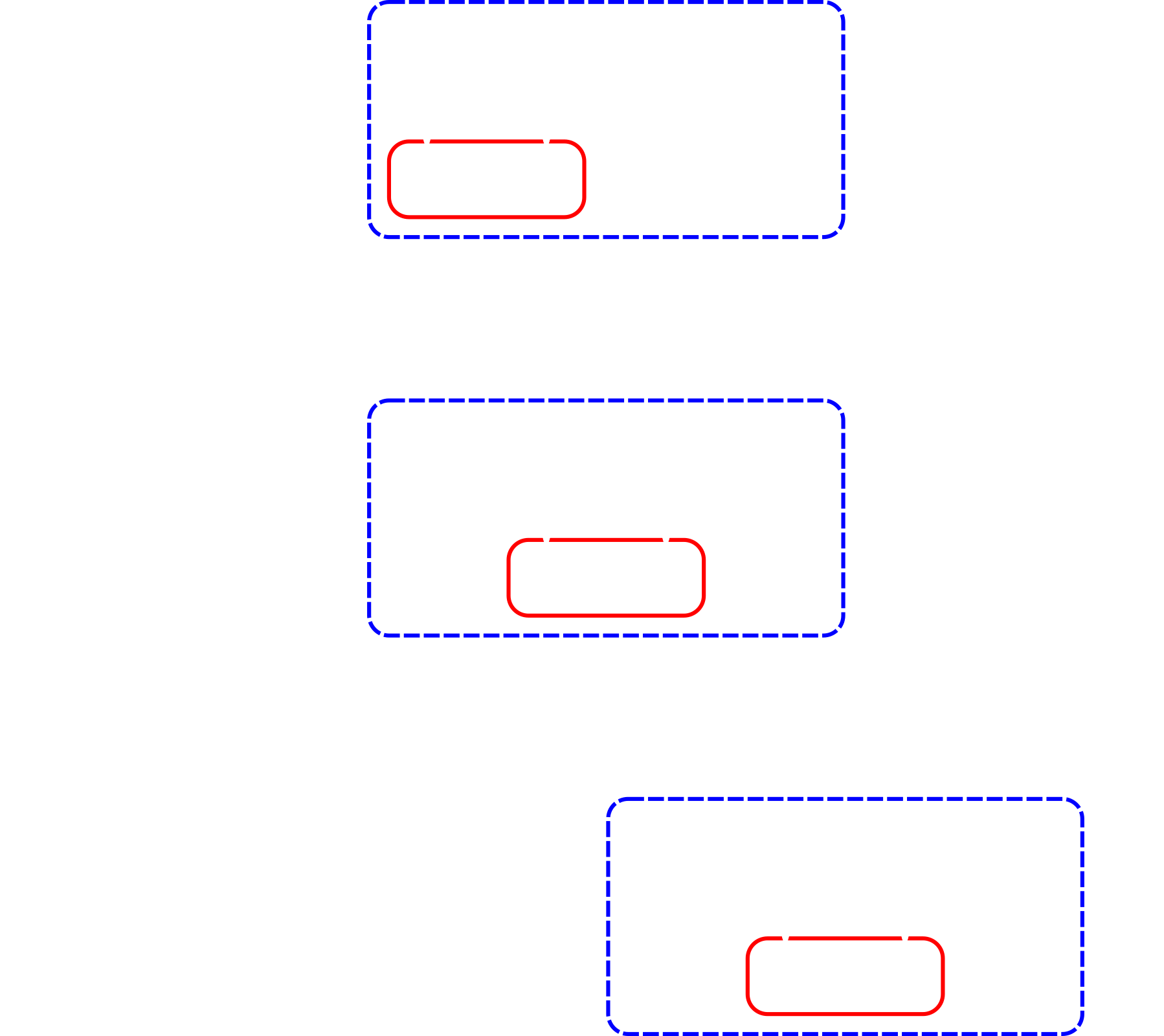
Run particle filter only on supported parameters.

50 qubit Ising chain, 8 qubit simulator, 4 qubit observable

Going Further

Hyperparameterization Granade et al. s87: $\Pr(d | y) = \expect_x[\Pr(d | x) \Pr(x | y)]$.
Allows composing w/ noise, inhomogeneity, etc.
Time-dependence Isard and Blake cc76f6: Adding timestep update allows learning stochastic processes.
Model selection Ferrie 7nt: Using acceptance ratio or normalizations enables comparing models.
Quantum filtering Wiebe and Granade 1512.03145: Rejection filtering can be quantized using Harrow et al. bcz3hc.

Thank you!

Welford's Algorithm

Can compute $\bar{x}$, $\Sigma$ from one sample at a time. Numerically stable.

$n, \bar{x}, M_2 \gets 0$.
For each sample $x$:

$n \gets n + 1$ Record # of samples
$\Delta \gets x - \mu$ Diff to running mean
$\bar{x} \gets \bar{x} + \Delta / n$ Update running mean
$M_2 \gets M_2 + \Delta (x - \bar{x})$ Update running var

Return mean $\bar{x}$, variance $M_2 / (n - 1)$.

Vector case is similar.

Rejection and Particle Filtering for Hamiltonian Learning

Rejection Sampling Isn't Enough

Example: Biased Coin $x = (p)$

Rejection Filtering (RejF)

Example: Phase Estimation, $x = (\phi)$

Applications

Example: Phase Estimation, $x = (\phi)$

Liu-West Resampler

Particle Filter

Useful for Hamiltonian models...

...as well as other QIP tasks.

Example: $\vec{x} =$ COSY / Crosstalk

Example: $\vec{x} =$ COSY / Crosstalk

Error Bars

Assessing Performance

Simulation Costs

PGH: Particle Guess Heuristic

50 qubit Ising chain, 8 qubit simulator, 4 qubit observable

Going Further

Thank you!

Welford's Algorithm