Practical Characterization and Control of Quantum Systems
Cassandra Granade
Institute for Quantum Computing
Joint Work with Christopher Ferrie, Nathan Wiebe, Ian Hincks, Troy Borneman and D. G. Cory
Slides and references are available at https://www.cgranade.com/research/talks/sandia-2014/.
References like 10/abc can be looked up using http://doi.org/abc. \(\renewcommand{\vec}[1]{\boldsymbol{#1}}\) \(\renewcommand{\matr}[1]{\mathbf{#1}}\) \(\newcommand{\bra}[1]{\left\langle#1\right|}\) \(\newcommand{\ket}[1]{\left|#1\right\rangle}\) \(\newcommand{\braket}[2]{\left\langle#1\mid#2\right\rangle}\) \(\newcommand{\dd}{\mathrm{d}}\) \(\newcommand{\ii}{\mathrm{i}}\) \(\newcommand{\ee}{\mathrm{e}}\) \(\newcommand{\expect}{\mathbb{E}}\) \(\newcommand{\matr}[1]{\mathbf{#1}}\) \(\newcommand{\T}{\mathrm{T}}\) \(\newcommand{\Cov}{\operatorname{Cov}}\) \(\newcommand{\Tr}{\operatorname{Tr}}\) \(\newcommand{\real}{\mathbb{R}}\) \(\renewcommand{\Re}{\operatorname{Re}}\)
Introduction
This talk will proceed in two parts:
- Using sequential Monte Carlo for practical characterization
- Extending optimal control theory algorithms to include realistic models of classical electronics
Part 1: Practical Characterization
Limits of Traditional Characterization
Quantum information experiments are pushing the limits of traditional characterization techniques.
- Large numbers of parameters to estimate.
- Errors in estimated parameters can be highly correlated.
- Can be hard to extract confidence and credible regions.
- Can be difficult to incorporate practical experimental effects.
Example: Hyperfine Measurement in NV Centers
Electronic spin \(\vec{S}\) in NV center coupled to a nearby carbon spin \(\vec{I}\): \[ H = \Delta_{\text{zfs}} S_z^2 + \gamma_e (\vec{B} + {\color{red} \vec{\delta B}}) \cdot \vec{S} + \gamma_C (\vec{B} + {\color{red} \vec{\delta B}}) \cdot \vec{I} + \vec{S} \cdot {\color{red} \mathbf{A}} \cdot \vec{I}, \]
\({\color{red} \vec{\delta B}}\) causes large errors in \({\color{red} \matr{A}}\), making it difficult to characterize \(H\) using spectroscopic methods.
Enabling Characterization with Simulation
Bayes' Rule relates estimation to simulation:
\[ \Pr(\text{hypothesis} | \text{data}) = \frac{\color{red}{\Pr(\text{data} | \text{hypothesis})}}{\Pr(\text{data})} \Pr(\text{hypothesis}) \]
The posterior distribution describes what we learn from our data about hypotheses.
\(\Rightarrow\) Practical characterization can be enabled using sequential Monte Carlo.
- Classical Bayesian algorithm
- Uses simulation to estimate parameters
- Numerical algorithm— doesn't assume analytic solution
For instance, to learn about a Hamiltonian \(H\) given a measurement \(d\):
\[\begin{align} \Pr(H) & \approx \sum_{i=0}^N w_i \delta(H - H_i) \\ \Pr(H | d) & \approx \sum_{i=0}^N w_i \delta(H - H_i) \times \Pr(d | H_i) / \mathcal{N} \end{align}\]
\(\mathcal{N}\): normalization factor (can be found implicitly)
Set \(w_i \gets w_i \Pr(d | H_i) / \mathcal{N}\) to be new prior.
- Iterative \(\Rightarrow\) SMC can be used online as data arrives.
- Also reduces overhead for postprocessing large datasets.
Estimate of \(H\) is then \[ \hat{H} = \expect[H] = \sum_i w_i H_i. \]
(Doucet et al., Stat. & Comp. 10 3 197-208; Huszár and Houlsby, PRA 85 052120; Granade et al. 10/s86, NJP 14 10 103013 10/s87)
Generality of Simulation-Based Characterization
Simulation \(\Pr(d|H_i)\) with hypothesis \(H_i\) allows for additional experimental details in our simulation, at the trade off of computational cost.
Examples:
- Finite and unknown \(T_1\), \(T_2\).
- Unknown visibility.
- Uncertainty in control fields.
Parameter Reduction
We often need not consider all possible Hamiltonians, but can consider a set of physically reasonable Hamiltonians.
Let \(H = H(\vec{x})\) be a parameterization, where \(\vec{x} \in \real^d\).
Example (Ising model):
\[ H(\vec{x}) = \sum_{\langle i,j \rangle} x_{i,j} \sigma_z^{(i)} \sigma_z^{(j)} \]
Prior Knowledge
SMC is Bayesian, and thus incorporates prior knowledge.
Modeled by a prior distribution \(\Pr(\vec{x}) := \pi(\vec{x})\).
Examples:
- Secondary experiment gives rough estimate of a parameter.
- Physical arguments place limits on feasible parameter values.
- Ab initio calculations give expected range for parameters.
Characterizing Uncertainty
Since we have the posterior, we can calculate the mean and covariance easily:
\[\begin{align} \expect[\vec{x}] & = \sum_i w_i \vec{x}_i \\ \Cov(\vec{x}) & = \expect[\vec{x}\vec{x}^\T] - \expect[\vec{x}]\expect[\vec{x}]^\T \end{align}\]
- SMC replaces integrals over \(\Pr(\vec{x})\) with finite sums.
- Covariance describes uncertainty in estimate.
Ambiguity in Approximation
xs, ys = multivariate_normal([0, 0], identity(2), size=(200,)).T
xs2, ys2 = 8 * np.random.random((2, 200)) - 4

figure(figsize=(12,6))
subplot(1,2,1); scatter(xs, ys); ylim(-4, 4)
subplot(1,2,2); scatter(xs2, ys2, s=norm.pdf(xs2) * norm.pdf(ys2) * 1000);

Avoiding Impoverishment
- The number of samples \(N\) must be large to represent \(\Pr(\vec{x} | \text{data})\).
- As more data is collected, posterior becomes sharper.
- Initial particles are unlikely to have support in posterior, reducing effective \(N\).
Solution: resampling. Replace SMC samples with different samples that better represent the same distribution.
Uses that information can be stored in weights \(\{w_i\}\) or positions \(\{\vec{x}_i\}\).
Liu-West Resampling Algorithm
- Sample new \(\vec{x}_i'\) from kernel density estimate such that \(\expect[\vec{x}]\) and \(\Cov(\vec{x})\) are preserved.
- Set new weights to uniform \(w_i' = 1/ N\).
Liu-West distribution: \[ \Pr(\vec{x}'_i) = \sum_i w_i \frac{1}{\sqrt{(2\pi)^k |\matr{\Sigma}|}} \exp\left( -\frac{1}{2} (\vec{x}' - \vec{\mu}_i)^\T \matr{\Sigma}^{-1} (\vec{x}' - \vec{\mu}_i) \right) \] where \[\begin{align*} \vec{\mu}_i & = a \vec{x}_i + (1 - a) \expect[\vec{x}] \\ \matr{\Sigma} & = (1- a^2) \Cov[\vec{x}] \\ a & \in [0, 1], \end{align*}\]
(West, J. Royal Stat B 55 2 409-422; Liu and West 2001)
Putting it Together: The SMC Algorithm
- Draw \(N\) "particles" \(\{\vec{x}\}_{i=0}^{N-1}\) from \(\pi(\vec{x})\).
- Set \(w_i = 1 / N\) for each particle.
For each new measurement \(d\):
- Let \(w_i \gets w_i \Pr(d | \vec{x}_i)\).
- Normalize \(w_i\) to be a distribution.
- If \(1 / \sum_i w_i^2 < 0.5 N\), resample.
(Doucet et al., Stat. & Comp. 10 3 197-208)
Software Implementation
prior = UniformDistribution([[0.9, 1], [0.4, 0.5], [0.5, 0.6]])
updater = SMCUpdater(
    RandomizedBenchmarkingModel(), 10000,
    prior, resampler=LiuWestResampler()
)

# As data arrives:
# updater.update(datum, experiment)
(Granade et al., arXiv:1404.5275; github.com/csferrie/python-qinfer)
Provides an infrastructure for rapidly deploying SMC. User defines:
- Parameterization of model and experiments
- Possible outcomes
- Likelihood of data
Built-In Plotting
updater.plot_posterior_contour(0, 1, res1=50, res2=50)

Built-In Plotting
updater.plot_posterior_marginal(0)
ylim(ymin=0)

Estimation
QInfer handles drawing estimates from the current SMC distribution:
print updater.est_mean()
print sqrt(diag(updater.est_covariance_mtx()))
print updater.est_entropy()
Region Estimation
Credible region \(X_{\alpha}\): \(\Pr(\vec{x} \in X_{\alpha}) \ge \alpha\)
Several ways to choose \(X_{\alpha}\):
- covariance ellipses— if approx. normal
- convex hulls— very general, but long description
- minimum volume enclosing ellipse (MVEE) for the hull— approximate, but easy to represent
cov = updater.est_covariance_mtx()
hull_faces, hull_vertices = updater.region_est_hull()
ellipse_mtx, ellipse_centroid = updater.region_est_ellipsoid()
State-Space Methods
SMC can also be used to track the state of a parameter that fluctuates in time.
Here, the true value of \(\omega\) is drawn from a Gaussian process. After each measurement, SMC particles are moved to track \(\omega\), \(\vec{x}(t_{k + 1}) \sim \mathrm{N}(\vec{x}(t_k), \sigma^2)\).
(Doucet and Johansen 2011)
Robustness of SMC: Finite Sampling
When using SMC without exact likelihoods, finite sampling of simulator introduces finite error \(\epsilon\):
\[ w_i \mapsto w_i (\Pr(d | \vec{x}_i) + \epsilon) / \mathcal{N} \]
Example (noisy coin): risk for 1000 experiments vs number of samples.

(Ferrie and Granade 2014, PRL 112 13 130402 10/tdj)
Robustness of SMC: Incorrect Model
We also want SMC to be robust against errors in the simulator. Below: risk when Ising simulator neglects terms of order \(10^{-4}\).

(Wiebe et al. PRA 89 4 042314 10/tdk)
Other Features
- Model selection and (coming soon) model-averaged estimation
- Parallelization with IPython
- Example of GPU-based model
- Improved resampling
- Robustness-testing tools (ex.: erroneous models)
Documentation
iframe("http://python-qinfer.readthedocs.org/en/latest/")
SMC and QInfer in Action: Randomized Benchmarking
Randomized benchmarking: apply random Clifford gates \(\{S_i\}\) to learn average fidelity of a gateset \(\{U_j\}\):

SMC and QInfer in Action: Randomized Benchmarking
- Fidelity exposed as decay of survival probability \(\Tr(ES_{\vec{i}}[\rho])\); removes effect of preparation \(\rho\) and measurement \(E\) (SPAM).
- Can interleave with gate of interest.
- Least-squares fitting often used to extract fidelity.

(Knill et al., PRA 77 1 012307 10/cxz9vm; Magesan et al., PRL 109 8 080505 10/s8j)
SMC and QInfer in Action: Randomized Benchmarking
SMC can be used to accelerate interleaved RB experiments.
- Interpret randomized benchmarking as a likelihood.
Example (zeroth-order model): \[ \Pr(\text{survival} | A, B, \tilde{p}, p_{\text{ref}}; m, \text{mode}) = \begin{cases} A (\tilde{p} p_{\text{ref}})^m + B & \text{interleaved} \\ A (p_{\text{ref}})^m + B & \text{reference} \end{cases} \]
- \(\tilde{p}\) and \(p_{\text{ref}}\): interleaved and reference depolarizing parameters (resp)
- \(A\) and \(B\): constants describing SPAM
Advantages:
- \(0 \le p_{\text{ref}}, \tilde{p} \le 1\) manifest in prior— avoids instability as \(\tilde{p} \to 1\).
- Using prior information and correlations between different data can drastically reduce data requirements.
SMC and QInfer in Action: Randomized Benchmarking
Straightfoward to implement in QInfer:
from qinfer.abstract_model import Model

class RandomizedBenchmarkingModel(Model):
    # ...

    def likelihood(self, outcomes, modelparams, expparams):
        p_tilde, p, A, B = modelparams.T[:, :, np.newaxis]

        p_C = p_tilde * p
        p = np.where(expparams['reference'][np.newaxis, :], p, p_C)

        m = expparams['m'][np.newaxis, :]

        pr0 = 1 - (A * (p ** m) + B)

        return Model.pr0_to_likelihood_array(outcomes, pr0)

    # ...
(Granade et al., arXiv:1404.5275)
SMC and QInfer in Action: Randomized Benchmarking


(Left: \(m = 1, 2, \dots, 100\); Right: \(10^3\) shots/sequence length, \(m = 1, 11, \dots, m_{\max}\))
SMC and QInfer in Action: Hyperfine Measurement
With SMC, we can easily integrate data from many different kinds of measurements and control parameters:
- Rabi, Ramsey and SPAM experiments
- Several different \(\vec{B}\) fields
Experimental variety is a resource for decorrelating errors in static controls from hyperfine parameters.
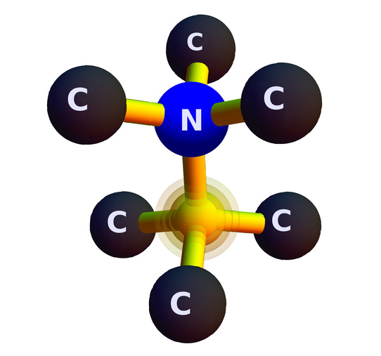
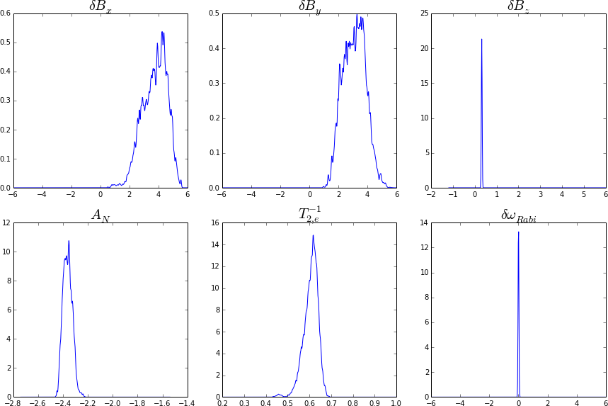
Electronic spin in an NV center coupled to a nitrogen spin: \[ H = \Delta_{\text{zfs}} S_z^2 + \gamma_e (\vec{B} + \vec{\delta B}) \cdot \vec{S} + \gamma_N (\vec{B} + \vec{\delta B}) \cdot \vec{I}_N + {A}_N S_z I_{N,z} \] Using 5000 particles, we can get accurate estimates of both \(\vec{\delta B}\) and \(\matr{A}_N\). Shown below for 163M total shots (about 300k photons).
Simulations show that we can hyperfine couplings to carbon spins as well:
Part 2: Control of Quantum Devices with Non-Linear Electronics
Pulse Engineering
Modern optimal control theory (OCT) algorithms allow for designing pulses with many desired properties, including
- Robustness to distributions over Hamiltonians
- Bandwidth and power limits
- Ringdown compensation
Utility functional: \[\begin{align*} \Phi(\vec{p}) & = \Tr(U_{\text{target}}^{\dagger} U(\vec{p})) / \dim^2\mathcal{H}, \text{where} \\ U(\vec{p}) & := \prod_{i=N}^{1} \ee^{-\ii \Delta t (H_0 + \sum_{k=1}^K p_{i,k} H_k)} \end{align*}\]
- \(H_0\): internal Hamiltonian
- \(\{H_k\}\): control Hamiltonians
- \(\Delta t\): timestep
GRAPE
Gradient-ascent pulse engineering (GRAPE) is a commonly used OCT algorithm.
- Provides fast evaluation of \(\vec{\nabla}\Phi\).
- Uses gradient-ascent or conjugate-gradient to maximize \(\Phi\).
However, GRAPE assumes linearity of classical control electronics (transfer function).
(Khaneja et al., JMR 172 2 296-305 10/cg8cdh)
Calculating Gradients
Khaneja gives the gradients wrt the controls \(\{p_k(t)\}\) in terms of unitary time steps:
\[\begin{align} \frac{\partial \Phi}{\partial p_k(t_j)} & = -2 \Re\left\{\braket{P_j}{\ii \Delta t\, H_k X_j} \braket{X_j}{P_j} \right\} \\ X_j & := U_j \cdots U_1 \\ P_j & := U_{j+1}^\dagger \cdots U_{n}^\dagger U_{\text{target}} \\ U_j & := \exp\left(-\ii \Delta t (H_0 + \sum_{k=1}^{K} p_k(t_j) H_k )\right) \end{align}\]
Nonlinear Conjugate Gradient Method
- Choose initial pulse \(\vec{p}\).
- Let \(\beta = 0\), \(\vec{s} = 0\).
- Until utility goal is met:
- Calculate \(\Phi(\vec{p})\), \(\vec{\nabla}\Phi(\vec{p})\).
- Update \(\beta\) using Polak–Ribière formula.
- \(\vec{s} \gets -\vec{\nabla}\Phi + \beta \vec{s}\).
- Search along \(\vec{s}\), \(\vec{p} + \alpha \vec{s}\) for a step size \(\alpha > 0\).
- \(\vec{p} \gets \vec{p} + \alpha \vec{s}\)
Gradient information used to update search directions, line search used to determine step sizes.
Example: Non-Linear Resonators
Superconducting resonators admit kinetic inductance \(L = L(I_L) = L_0 (1 + \alpha_L \|I_L\|^2)\) and a nonlinear resistance \(R = R(I_R) = R_0 (1 + \alpha_L \|I_R\|^\eta)\).

(Maas 2003; Benningshof et al., JMR 230 84-87 10/s8m; Mohebbi et al., JAP 115 9 094502 10/s8n)
Therefore, the resonance frequency, quality factor and coupling are all functions of current, frustrating linear approximations.
Distortions
Let \(\vec{p}\) be a discretization of \(p_k(t)\). Then, the effect of classical electronics (e.g.: a high-\(Q\) resonator) can be modeled as an operator \(g : \vec{p} \mapsto \vec{q}\).

Since \(\vec{\nabla}_\vec{p}\Phi(g[\vec{p}]) = \vec{\nabla}_\vec{q}\Phi(\vec{q}) \cdot J_g(\vec{p})\), if we can find the Jacobian of a distortion operator, we can include it into GRAPE.
- Control search is thus for un-distorted pulse.
- Can get higher fidelity controls by including distortion.
- Allows driving at higher powers— don't need to limit to linear regime.
Simulation of Non-Linear Control Systems
Including the nonlinear inductance and resistance gives us a system of differential equations \[\begin{align} \frac{\dd}{\dd t} \left[\begin{matrix} I_L \\ V_{C_m} \\ V_{C_t} \end{matrix}\right] & = \matr{A}(I_L, I_R) \left[\begin{matrix} I_L \\ V_{C_m} \\ V_{C_t} \end{matrix}\right] + \vec{y} V_s(t), \end{align}\] where \(\matr{A}\) and \(\vec{y}\) describe the circuit and driving term, respectively.
This system is nonlinear since \(\matr{A} = \matr{A}(I_L, I_R)\).
Note: rescaling the driving term does not just rescale the output current.
Simulation of Non-Linear Control Systems
To simulate the distortion introduced by this system, we let \(g : \vec{V}_s \mapsto \vec{I}_L\) be the solution to the DEs for a given driving term.
The Jacobian can then be approximated perturbatively, \[ \frac{\partial g_{m,l}}{\partial p_{n,k}} \approx \left[\frac{g(\vec{p} + \epsilon \vec{e}_{n,k}) - g(\vec{p})}{\epsilon}\right]. \]
Taking a small \(\epsilon\) allows us to find a good direction for the conjugate gradient step.
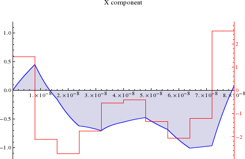
Example: Finding a \(\pi/2)_x\) Gate
For a strongly non-linear resonator, we find the following 99.1% fidelity \(\pi/2)_x\) gate using GRAPE. The un-distorted pulse is shown in red.


Robustness to Distributions
We want to relax that \(H_0\) and \(\{H_k\}\) be known with certainty.
Let \(\overline{\Phi} = \expect_{H_0, \{H_k\}}[\Phi]\)
- \(H_0\): internal
- \(\{H_k\}\): control
By linearity of \(\expect\): \[ \vec{\nabla}_\vec{p} \overline{\Phi}(g[\vec{p}]) = \expect_{H_0, \{H_k\}} [\vec{\nabla}_{\vec{q}} \Phi(\vec{q})] \cdot J_g(\vec{p}) \]
To optimize pulses for \(\overline{\Phi}\), we represent \(\Pr(H_0, \{H_k\}) =: \Pr(H_0(\vec{x}), \{H_k(\vec{x})\}) \approx \sum_i w_i \delta(\vec{x} - \vec{x}_i)\).
Robust GRAPE thus can take an SMC approximation as input.
(Borneman et al., JMR 225 120-129 10/cksg3v)
Ringdown Optimization and Heuristic
Decay dominated by \(\ee^{-t / t_c}\), even in non-linear case. Can add a timestep \(p(t_{i+1}) = -g[\vec{p}](t_i)/(\ee^{\delta t / t_c} - 1)\) to drive pulse ringdown to zero.
- For non-linear, only an approximation.
- Multiple steps or optimization can improve ringdown compensation.
Using two timesteps for compensation:
(Borneman and Cory, JMR 207 2 220-233 10/s8p)
Putting it Together: Robust Pulses for Non-Linear Resonators

Conclusions
- Bayesian methods allow for including prior information in characterization
- Simulation is a resource for inference
- SMC allows for using Bayesian inference in a practical manner
- Robust to common errors (finite sampling, approximations in simulation)
- Can extend GRAPE with simulations of classical systems
- Allows for control of even strongly non-linear devices
- GRAPE can optimize over SMC-like distributions for practical control.
References
Full reference information is available on Zotero.
iframe('https://www.zotero.org/cgranade/items/collectionKey/VSWSNCCA')