Practical Bayesian Tomography
Cassandra E. Granade
Centre for Engineered Quantum Systems
joint work with Joshua Combes and D. G. Cory • [1509.03770](https://scirate.com/arxiv/1509.03770)
https://www.cgranade.com/research/talks/sqip-workshop/12-2015/
$
\newcommand{\ee}{\mathrm{e}}
\newcommand{\ii}{\mathrm{i}}
\newcommand{\dd}{\mathrm{d}}
\newcommand{\id}{𝟙}
\newcommand{\TT}{\mathrm{T}}
\newcommand{\defeq}{\mathrel{:=}}
\newcommand{\Tr}{\operatorname{Tr}}
\newcommand{\Var}{\operatorname{Var}}
\newcommand{\Cov}{\operatorname{Cov}}
\newcommand{\rank}{\operatorname{rank}}
\newcommand{\expect}{\mathbb{E}}
\newcommand{\sket}[1]{|#1\rangle\negthinspace\rangle}
\newcommand{\sbraket}[1]{\langle\negthinspace\langle#1\rangle\negthinspace\rangle}
\newcommand{\Gini}{\operatorname{Ginibre}}
\newcommand{\supp}{\operatorname{supp}}
\newcommand{\CC}{\mathbb{C}}
$
Citations are listed by handle (e.g. 10/abc or 10012/abc) or arXiv number.
handle $\mapsto$ https://dx.doi.org/handle
Even Bigger Models
- **Gate set tomography**: Still more parameters, but explicitly models multiple processes and prep/meas errors.
Let's Meet In the Middle
\[ \text{tomography} = \{ \text{state tomography}, \text{process tomography} \} \]
Tomography is exponentially hard, but is still essential for *small* quantum systems.
Sure, tomography, but why Bayesian?
- Gives calculus for including the effect of prior assumptions. - Good numerical algorithms. (More on this later!)
The Five Habits of Highly Effective Tomographic Procedures
- Provide accurate estimates. - Characterize their uncertainty. - Allow inclusion of prior knowledge. - Can track changes with time. - Come with “off-the-shelf” implementations.
We get the first two for free from taking a Bayesian perspective.
Challenges for Bayesian Tomography
- What prior should we use? - How should we update estimates in time? - How can we efficiently implement Bayesian tomography?
In this talk, we will address all three challenges.
But first,
A Short Primer on Bayesian Inference and Tomography
See also: - Jones [10/fpbsfw](https://dx.doi.org/10/fpbsfw) - Blume-Kohout [10/cn772j](https://dx.doi.org/10/cn772j)
Bayesian Parameter Estimation
Suppose we want to learn $x$ from data $D$. Then \[ \Pr(x | D) = \frac{\Pr(D | x)}{\Pr(D)} \Pr(x) \] is the posterior distribution over $x$.
$\Pr(x | D)$ describes what we know about $x$.
Likelihood Functions
$\Pr(D | x)$ is a likelihood function that specifies an experimental model.
For state tomography, our likelihood is Born's rule, \[ \Pr(E | \rho) = \Tr[E \rho], \] where $x = \rho$ is a state and $D = E$ is a measurement effect.
We estimate $\rho$ by the expectation value \[ \hat{\rho} = \expect[\rho | D] = \int \rho\,\Pr(\rho|E)\, \dd \rho. \]
This estimator is optimal for the mean squared error (Blume‑Kohout and Hayden quant-ph/0603116).
More generally, for all Bregman divergences (Banerjee et al. 10/d6cxmr).
We estimate the error incurred by our estimate $\hat{\rho}(E)$ in the same way: \begin{align*} & \expect[\Tr\left( (\rho - \hat{\rho}(E))^2 \right) | \text{data}] \\ =\ &\expect[\Tr\left( (\rho - \expect[\rho | E])^2 \right) | \text{data}] \\ =\ & \Tr\Cov(\rho | E). \end{align*}
More generally, \[ \hat{f} = \expect[f(\rho) | E]. \]
For state tomography, the Bayesian mean estimate is approximately optimal for the fidelity (Kueng and Ferrie [1503.00677](https://arxiv.org/abs/1503.00677)).
The error in an observable $X$ is given by the covariance superoperator $\Sigma\rho \mathrel{:=} \Cov(\sket{\rho})$. (Blume-Kohout 10/cn772j)
The Choi-Jamiołkowski isomorphism lets us rewrite process tomography as (ancilla-assisted) state tomography.
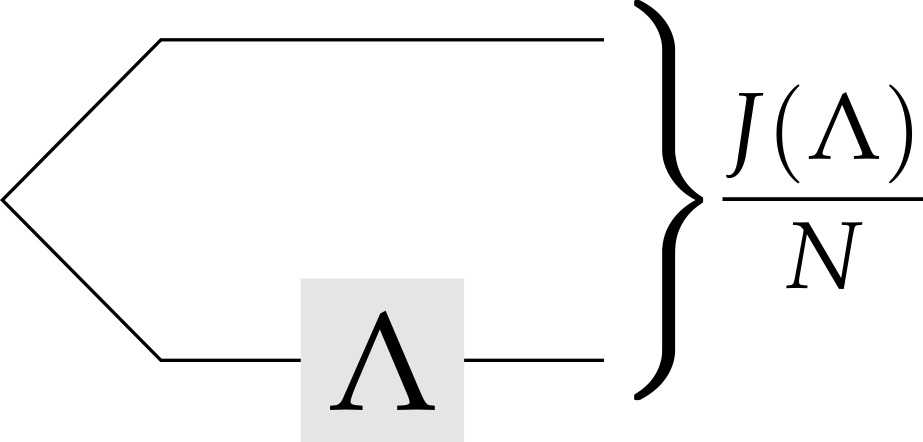
\[ \Tr[E \Lambda(\rho)] = \Tr[(\id \otimes E) J(\Lambda) (\rho^\TT \otimes \id)] = \sbraket{\rho^\TT, E | J(\Lambda)} \]
Thus, Bayesian inference allows us to estimate states $\rho$ and processes $\Lambda$.
What About The Prior?
Want conjugate priors $f(x; y)$ to perform Bayesian inference: \begin{align*} \frac{\Pr(d | x)}{\Pr(d)} f(x; y) = f(x; y'(d, y)). \end{align*} Inference then consists of finding a “nice” form for $y'$.
Examples
- Gaussian priors are conjugate for Gaussian likelihoods - Gaussian priors are *approximately* conjugate for one-qubit Hamiltonian learning (Ferrie *et al.* [10/tfx](https://dx.doi.org/10/tfx)) - Beta distribution is conjugate for coin estimation
Frustrating to find conjugate priors for states that respect Hilbert space structure.
Wait, Beta Distribution?
The beta distribution is supported on $[0, 1]$ for all $\alpha, \beta > 0$ and is a conjugate prior to the binomial distribution.
We will use later that the beta distribution is always supported on 0.
In practice, Bayesian mean estimation is not tractable in the exact case. We thus use particle filtering to approximate.
- Huszár and Houlsby [10/s86](https://dx.doi.org/10/s86) - Ferrie [10/7nt](https://dx.doi.org/10/7nt)
Implemented by the [QInfer library](https://github.com/csferrie/python-qinfer) for Python.
Particle Filtering for Approximate Estimation
\begin{align} \Pr(\rho) & \approx \sum_{p\in\text{particles}} w_p \delta(\rho - \rho_p) \\ w_p & \mapsto w_p \times \Pr(E | \rho_p) / \mathcal{N} \end{align}
Mixtures of $\delta$-functions are conjugate priors for practically any likelihood.
Big advantage: we only need samples from the prior!
As we collect data, this becomes unstable, so we must resample.
Particle filtering is used in a range of quantum information applications.
- Hamiltonian learning: Granade *et al.* [10/s87](https://dx.doi.org/10/s87), Stenberg *et al.* [10/7nw](https://dx.doi.org/10/7nw) - Randomized benchmarking: Granade *et al.* [10/zmz](https://dx.doi.org/10/zmz) - Quantum Hamiltonian learning and bootstrapping: Wiebe *et al.* [10/tdk](https://dx.doi.org/10/tdk), Wiebe *et al.* [10/7nx](https://dx.doi.org/10/7nx) - Phase estimation: Wiebe and Granade [1508.00869](https://arxiv.org/abs/1508.00869)
(A few more examples: Granade [10012/9217](https://dx.doi.org/10012/9217))
Why Particle Filtering?
(You Forgot My Favorite Algorithm)
- MCMC: works, but isn't streaming or time-dependent. - Rejection filtering (Wiebe and Granade [1508.00869](https://arxiv.org/abs/1508.00869)): only keeps sufficient statistics; need more expressive instrumental distribution.
Other Advantages
Expressing as Bayesian parameter estimation / particle filtering problem affords us a few other advantages.
Region Estimation
A credible region $R_\alpha$ for $\rho$ satisfies \[ \Pr(\rho \in R_{\alpha} | D) \ge \alpha. \]
Construct from particle approximation to posterior, covariance regions (Granade *et al* [10/s87](https://dx.doi.org/10/s87)), convex hull or minimum-volume enclosing ellipse (Ferrie [10/tb4](https://dx.doi.org/10/tb4)).
Built-in to QInfer.
Model Selection
- Akaike / Bayesian information criterion: Guţă *et al.* [10/7nz](https://dx.doi.org/10/7nz), van Enk and Blume-Kohout [10/7n2](https://dx.doi.org/10/7n2) - Bayes factors: Wiebe *et al.* [10/tdk](https://dx.doi.org/10/tdk) \begin{equation} \text{BF}(A : B) = \frac{\Pr(A | \text{data})}{\Pr(B | \text{data})} \end{equation} - Model averaging: Ferrie [10/7nt](https://dx.doi.org/10/7nt)
Bayes factor–based model selection built-in to QInfer.
Hyperparameterization
\begin{align*} \text{Suppose } \vec{x} & \sim \Pr(\vec{x} | \vec{y}) \\ \text{Then, } \Pr(D | \vec{y}) & = \expect_{\vec{x} | \vec{y}} [\Pr(D | \vec{x}, \vec{y})] \\ & = \int \Pr(D | \vec{x}, \vec{y}) \Pr(\vec{x} | \vec{y})\,\dd\vec{x}. \end{align*} Marginalizing gives us a likelihood for the hyperparameters $\vec{y}$!
Allows us to include effects outside of Born's rule. For instance, non-Cauchy decoherence (Granade et al. 10/s87).
But how do we choose our prior? Let's get to the meat of things.
Informative Priors for Bayesian Tomography
In order to be useful, a prior over states should: - Have support over all states, - Allow us to encode our assumptions, and - Be efficient to draw samples from.
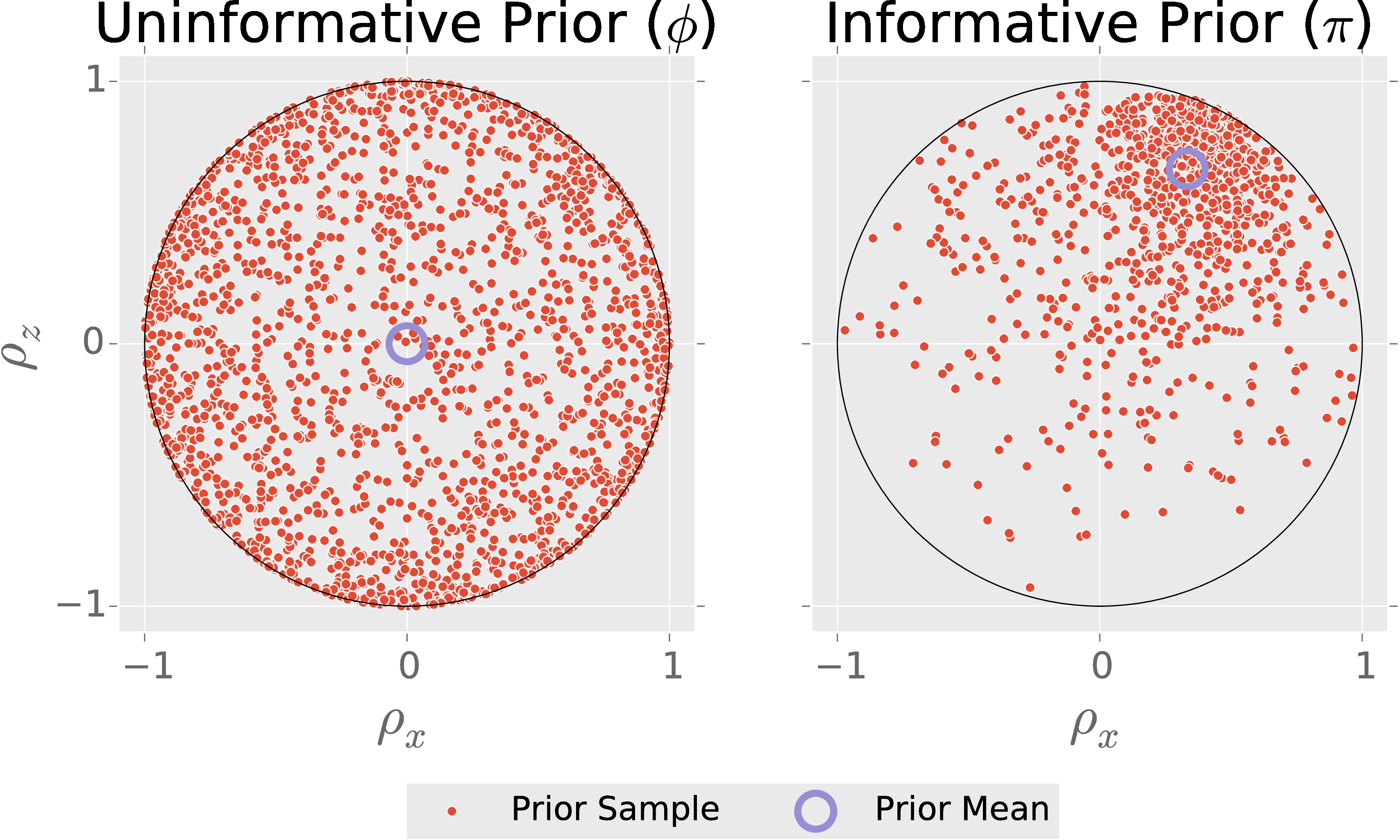
It helps to consider an uninformative prior first.
Ginibre Prior for Pure and Mixed States
- Let $X$ be a $N \times K$ matrix with complex Gaussian entries.
- $\rho \gets XX^\dagger / \Tr(XX^\dagger)$.
$\rank(\rho) = K$. If $K = 1$, $\rho$ is pure. If $K = N$, Hilbert-Schmidt prior.
NB: Choosing $X$ to be real gives Ginibre over redits.
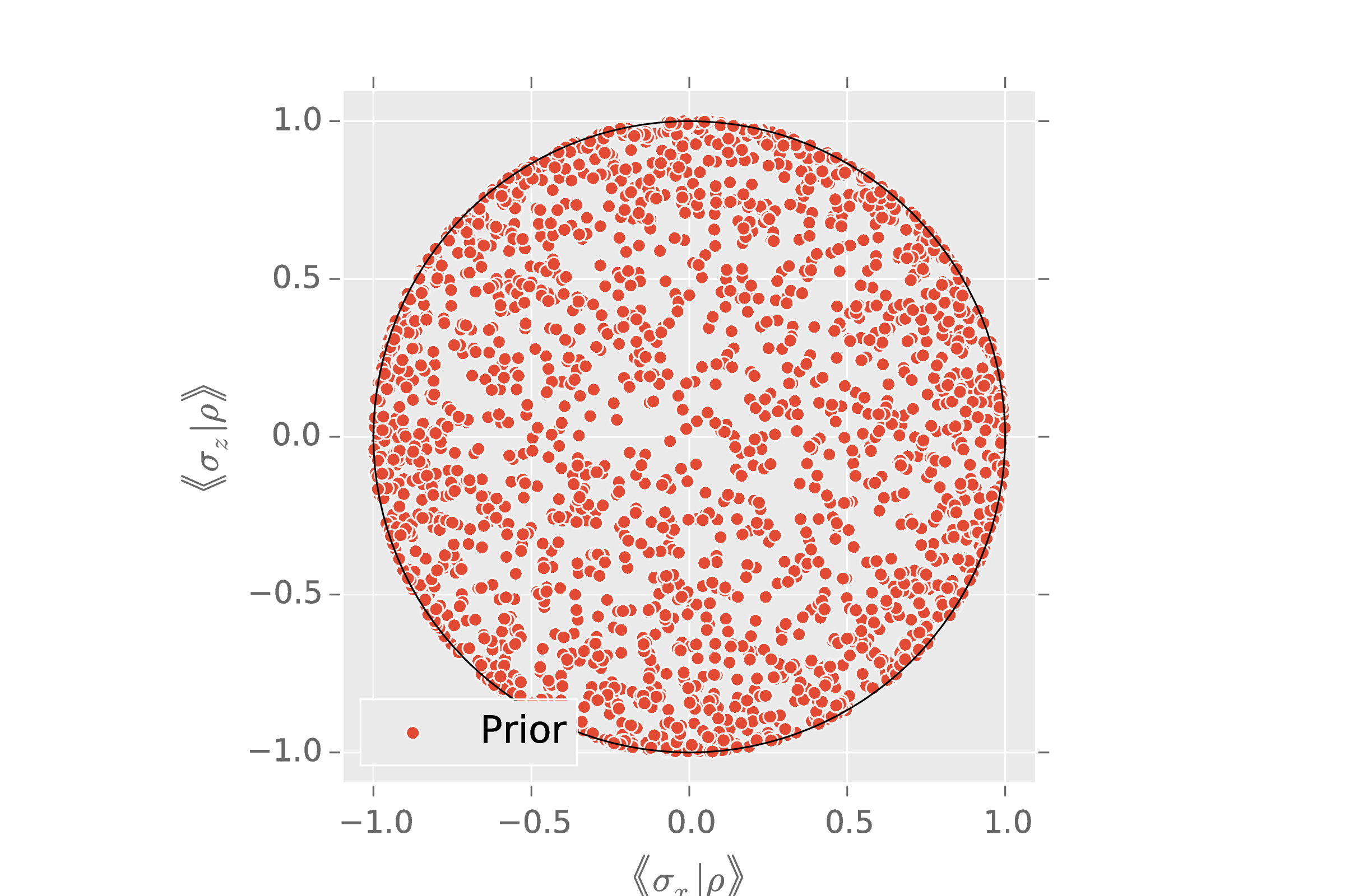
import qinfer as qi

basis = qi.tomography.pauli_basis(1)
prior = qi.tomography.GinibreReditDistribution(basis)
qi.tomography.plot_rebit_prior(prior, rebit_axes=[1, 3])
What makes $\Gini(N, K)$ uninformative? \[ \expect[\rho] = \id / N. \] The mean is the maximally-mixed state.
Other Useful Priors
- Haar, uniform over pure states - Bures, uniform over mixed states - BCSZ, uniform over CPTP maps
How do we add information to the prior, specifically the prior estimate state $\rho_\mu$?
Big idea: Use an ensemble of amplitude damping channels to transform a uniform prior.
Let $\phi$ be a fiducial prior. Then, for scalars $\alpha,\beta$ and a state $\rho_*$, draw $\rho_{\text{sample}}$ by:
- Draw $\rho \sim \phi$.
- Draw $\epsilon \sim \mathrm{Beta}(\alpha, \beta)$.
- $\rho_{\text{sample}} \gets (1 - \epsilon) \rho + \epsilon \rho_*$
NB: $\supp \pi \supseteq \supp \phi$
Choose $\rho_*$ s. t. $\expect_{\rho\sim\pi}[\rho] = \rho_\mu$:
\[ \rho_* = \left(\frac{\alpha + \beta}{\alpha}\right) \left( \rho_\mu - \frac{\beta}{\alpha+\beta} \frac{\id}{N} \right) \]
Choose $\alpha,\beta$ s. t. $\expect[\epsilon]$ is minimized: \[ \alpha = 1 \qquad \beta = \frac{\lambda_\min}{1 - N \lambda_\min}, \] where $\lambda_\min$ is the smallest eigenvalue of $\rho_\mu$.
That is, we contract the fiducial prior as little as possible to obtain the desired mean.
This construction preserves the support of our “flat” prior, takes $\rho_\mu$ as an input and can be easily sampled.
Inherits other assumptions by convexity (e.g.: rebit, CPTP, positivity, etc.).
Easy to Use
import qinfer as qi
import qutip as qt

I, X, Y, Z = qt.qeye(2), qt.sigmax(), qt.sigmay(), qt.sigmaz()
prior_mean = (I + (2/3) * Z + (1/3) * X) / 2

basis = qi.tomography.pauli_basis(1)
fiducial_prior = qi.tomography.GinibreReditDistribution(basis)
prior = qi.tomography.GADFLIDistribution(fiducial_prior, prior_mean)
QInfer's tomography support is backed by QuTiP.
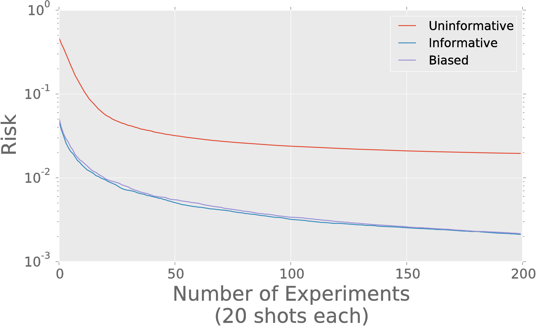
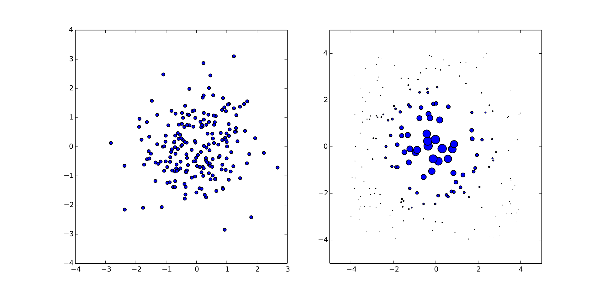
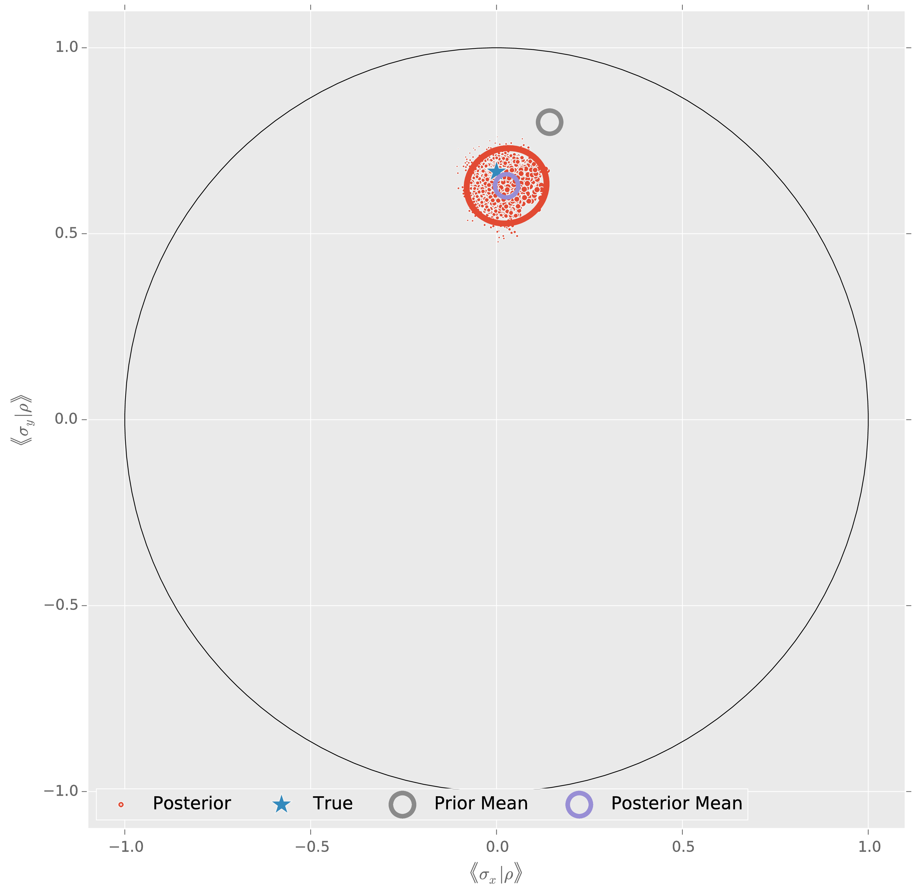
Prior Information Really Helps
Posterior covariance characterizes uncertainty.
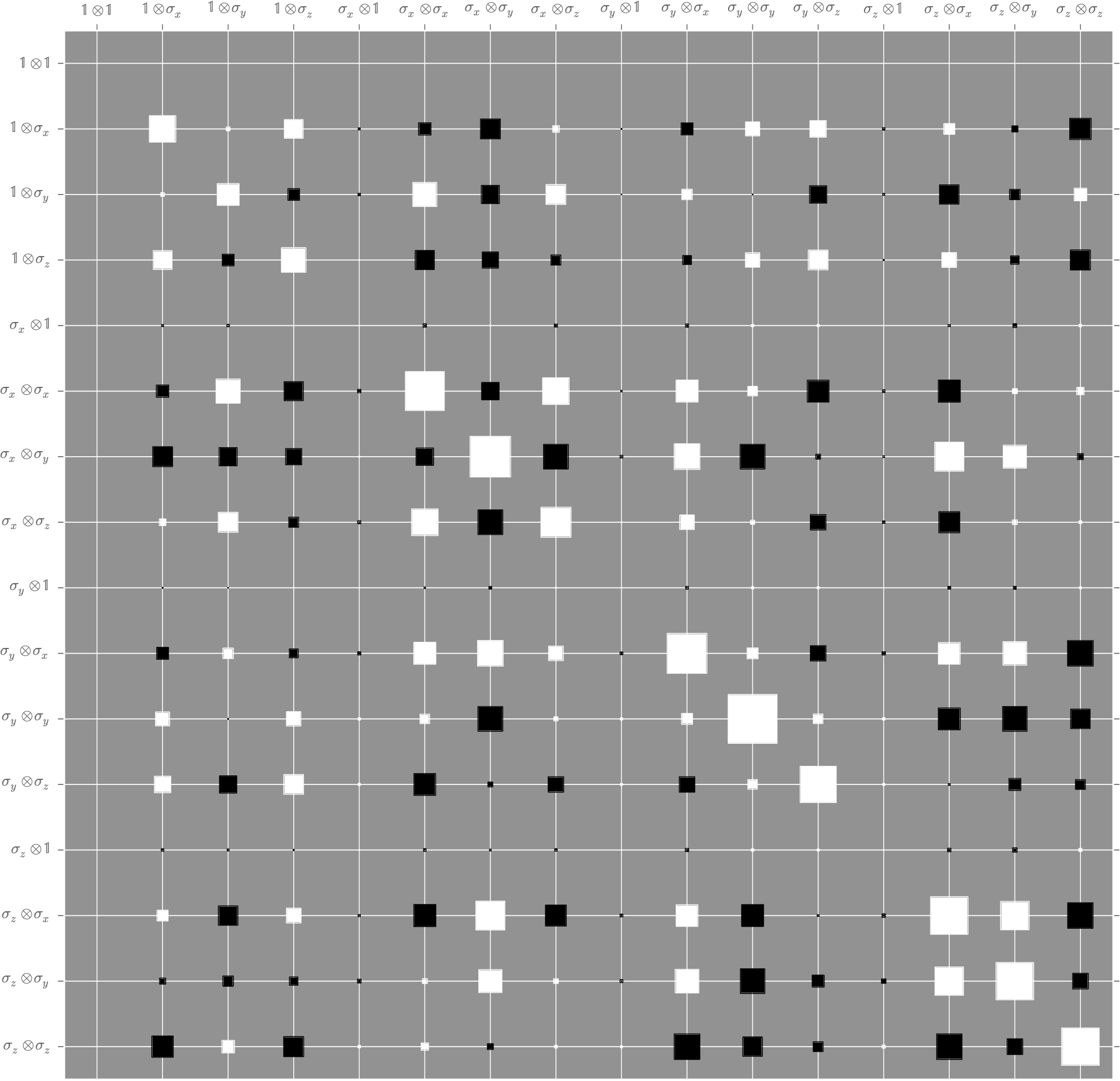
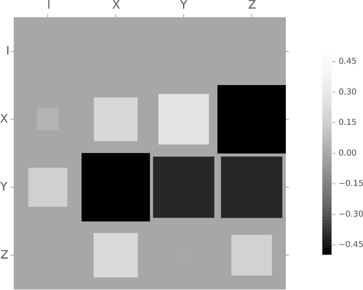
Principal channels tell us which components dominate our uncertianty.
How Do I Use This Bloody Thing?
(a quick tutorial)
All models are wrong, some are useful. —Chris Ferrie
(Box said it first, but it's funnier this way.)
We've seen how to create bases and priors, to finish we need a model, an updater and a heuristic.
model = qi.BinomialModel(qi.tomography.TomographyModel(basis))
The sequential Monte Carlo updater performs Bayes updates using particle filtering.
updater = qi.smc.SMCUpdater(model, 2000, prior)
heuristic = qi.tomography.RandomPauliHeuristic(updater,
    other_fields={'n_meas': 40}
)
This heuristic measures random Paulis 40 times each.
I'm Sick of This— Let's Measure!
for idx_exp in xrange(50):
    experiment = heuristic()

    # This is where your data goes! 💗
    # For now, we'll simulate. 💔
    datum = model.simulate_experiment(true_state, experiment)

    updater.update(datum, experiment)
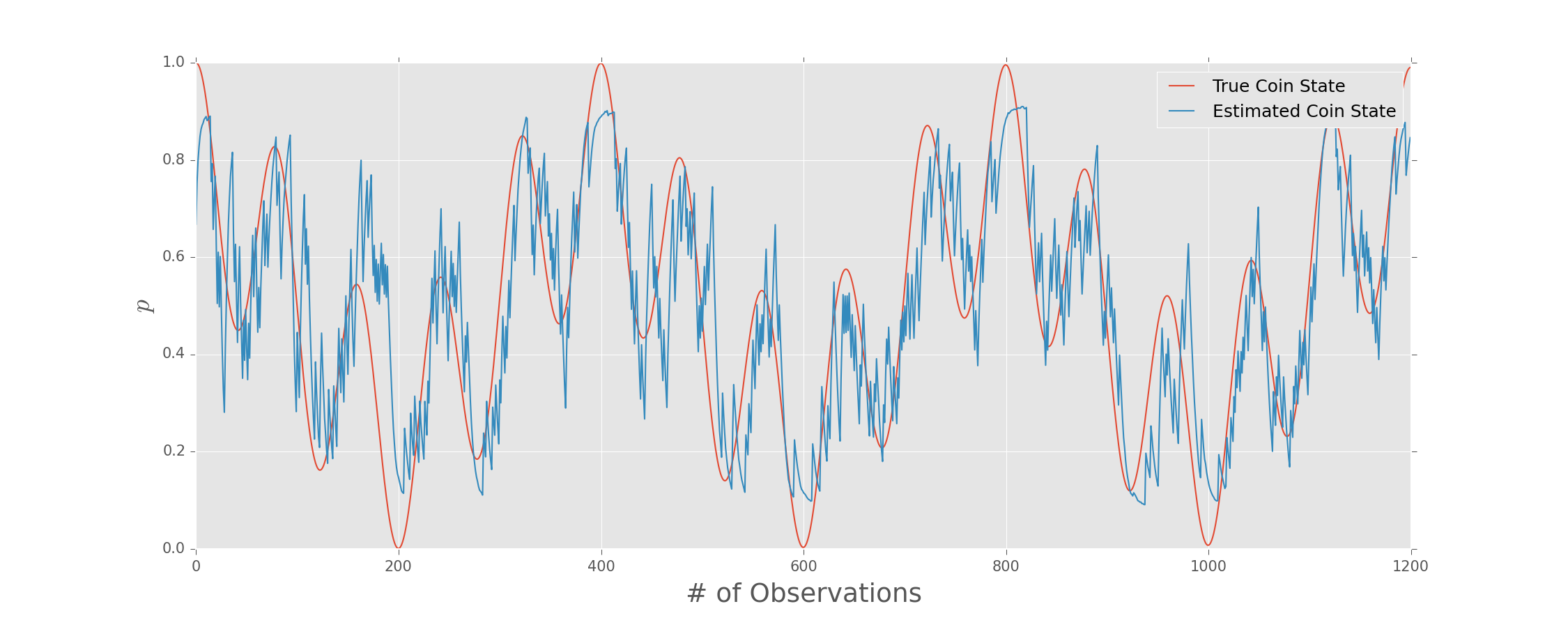
Tracking Time-Dependent States
Condensation Algorithm
Interlace Bayesian updates with diffusion \[ \rho(t_{k+1}) = \rho(t_k) + \Delta \eta. \] and truncation.
Draw each traceless parameter of the diffusion step $\Delta \eta$ from a Gaussian.
(Isard and Blake [10/cc76f6](https://dx.doi.org/10/cc76f6))
We can do this in general.
Parameterize a state $\rho$ as a real vector $\vec{x}$, \[ x_i = \sbraket{B_i | \rho} = \Tr(B_i^\dagger \rho), \] where $\{B_i\}$ is a basis of Hermitian operators.
By convention, $\Tr(B_i) = \delta_{i0} / \sqrt{D}$. E.g.:
- Pauli basis
- Gell-Mann basis
Co-Evolution for Fun and Diffusion Estimation
We don't need to assume a particular diffusion rate. Include as model parameter $\eta$, such that \begin{equation} \sigma = \sqrt{t_{k + 1} - t_k} \eta. \end{equation}
Bayesian updates on the state then “co-evolve” $\eta$ to learn diffusion rate.
We don't need to assume that the "true" state follows a random walk.
Conclusions
- New prior for quantum states and channels - Complete software implementation for Bayesian tomography - Time-dependence for quantum state tomography
These advances help make Bayesian tomography practical for modern experimental practice.