Characterizing and Verifying 100-Qubit Scale Quantum Computers¶

Cassandra Granade
Institute for Quantum Computing¶

https://www.cgranade.com/research/talks/unm-2014 \(\renewcommand{\vec}[1]{\boldsymbol{#1}}\) \(\newcommand{\ket}[1]{\left|#1\right\rangle}\)

Joint Work with Nathan Wiebe, Christopher Ferrie, Ian Hincks, Rahul Deshpande and D. G. Cory

Quantum Computing at the 100 Qubit Scale¶

In order for quantum computing to be useful, we need to be able to build, characterize and verify quantum devices at scales well past current techniques.

In this talk, I will focus on learning the Hamiltonian dynamics of large quantum systems, at scales approaching 100 qubits.

Characterization algorithms must be efficient.¶

• As we approach 100 qubits, the costs of characterization become more important.
• Must be able to characterize with modest numbers of measurements and computational resources.

Characterization must use prior information.¶

• Exponentially many parameters are needed to describe the dynamics of a quantum system in full generality.
• Prior information about the form of the dynamics must be used to restrict the number of parameters that must be learned.
• [HW12] show that adaptivity on prior information can be necessary for obtaining optimal error scaling.

Algorithms must serve experimental concerns.¶

• Characterization must include experimental noise and effects, or else it will not be useful in practice.
• No experiment is described by a Hamiltonian alone.
• Experimental description also includes a description of how control, preparation and readout are implemented.
• Adaptive characterization algorithms must integrate with experimental control systems in order for adaptiveness to be useful.

Algorithms must be generic.¶

• Not clear yet which modalities will be most useful.
• Not clear what the most interesting applications will be.
• Algorithms must be generic enough to be applicable to a wide range of systems and applications.

Characterization must be robust.¶

• In addition to experimental noise, characterization algorithms must be robust to simulation and numerical errors.
• Useful conclusions must be reached with the use of physically realistic resources.

Characterization must enable verification.¶

• Once we are able to build a 100-qubit scale device, we must be able to assert that it works as intended.
• Especially difficult given the limits of our ability to classically simulate the dynamics of large quantum systems.

Characterization Algorithms¶

The characterization of quantum systems is a rich field.

We start by reviewing a few approaches, their advantages, and what prevents them from being applicable at the 100-qubit scale.

Traditional Tomography¶

State and process tomography can be used iteratively to probe Hamiltonian dynamics.

• Few assumptions required.
• Requires exponentially many parameters in the size of the system.
• Reconstruction of \(H\) from \(e^{-i H t}\) need not be efficient or numerically stable.

Robust Lindblad Estimation¶

• Uses quantum dynamical semigroup assumption to considerably reduce model dimension.
• Still exponentially many parameters.

[BH+03]

Randomized Benchmarking¶

• Efficiently extracts information about the fidelity of a gate.
• Separates gate fidelity from SPAM errors.
• Only produces estimate of the fidelity; does not produce a full characterization.

[MGE12]

Gate Set Tomography¶

• Requires less assumptions (no need to know input state or measurement).
• Assumptions can be relaxed further, at added expense.
• Provides rigorous separation between model and data.
• In general, can be more expensive than traditional tomography.

[BG+13]

Local Hamiltonian Learning by Short-Time Evolution¶

• Uses locality assumption together with Lieb-Robinson bounds to guarantee scaling of errors and exponentially reduce the number of parameters.
• Requires numerically unstable matrix inversion.
• Information content of short-time measurements is bounded by the Fisher information, \(I \in O(t^2)\).
• Short-time evolution thus requires exponentially many measurements.

[dSLP11]

Simulation and Characterization¶

We can build upon these techniques by exploiting a key insight from Bayesian inference: simulation is a resource for characterization.

To see this, suppose that we have a probability \(\Pr(d | H)\) of obtaining data \(d\) from a system whose Hamiltonian is \(H\). Then, by Bayes' rule,

A Way Forward to 100-Qubit Scale Characterization¶

This is very powerful, as it allows us to bring our best simulation resources to bear on the problem of characterizing large quantum systems.

Importantly, \(\Pr(d | H)\) need not be a classical simulation, but can be implemented using quantum resources. This will then enable us to use a known quantum system as a tool to verify the dynamics of a system under study.

Outline¶

In the rest of this talk, I will describe:

• An algorithm that uses classical simulation to characterize quantum systems,
• How this algorithm can be extended to use quantum resources,
• The robustness of our algorithm, and
• An example of an experiment that demonstrates the utility of our approach.

Characterization with Classical Resources¶

Quantum Characterization as Parameter Estimation¶

To build our approach, we express the problem of characterizing quantum systems as one of parameter estimation. Thus, instead of reasoning directly about the Hamiltonian \(H\), we consider a parameterization \(\vec{x}\) such that \(H = H(\vec{x})\). This offers two distinct advantages:

Dimension Reduction¶

The dimension of \(\vec{x}\) can be substantially smaller than that of \(H\) by restricting the parameterization to a specific model.

Experimental Relevance¶

We can also include in \(\vec{x}\) not just Hamiltonian parameters, but also parameters describing the details of a particular implementation.

For example:

• \(T_2\)
• Visibility of measurements
• Polarization of initial states
• Uncertainty in applied control

Example: Hyperfine Couplings in NV Centers¶

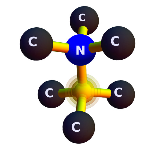
Image courtesy of Ian Hincks.

In NV centers, the electron spin degree of freedom \(\vec{S}\) couples to a \({}^{13}\text{C}\) spin \(\vec{I}\) by a hyperfine interaction, such that

\[ H = \Delta_{\text{zfs}} S_z^2 + \gamma_e \vec{B} \cdot \vec{S} + \gamma_C \vec{B} \cdot \vec{I} + \vec{S} \cdot \mathbf{A} \cdot \vec{I}, \]

where \(\vec{B}\) is the magnetic field, and where \(\Delta_{\text{zfs}}\) is the zero-field splitting.

Let \(\vec{B} = \vec{B}_0 + \delta \vec{B}\), where \(\delta \vec{B}\) is an unknown error in setting the magnetic field. Moreover, choose the coordinate system such that \[ \mathbf{A} = \left( \begin{matrix} A_{xx} & 0 & A_{xz} \\ 0 & A_{yy} & 0 \\ A_{xz} & 0 & A_{zz} \end{matrix} \right) \] contributes four real parameters.

• Given an evolution time \(\tau\) and a field setting \(\vec{B}_0\), the data generated by the Ramsey experiments can then be described using parameters \(\vec{x} = (\delta \vec{B}, \mathbf{A}, \alpha, \beta, T_{2,c}^{-1}, T_{2,e}^{-1})\), where \(\alpha\) and \(\beta\) describe the visibility of the single-shot readout.

A Bayesian Approach to Parameter Estimation¶

Having adopted a parameterization \(\vec{x}\), at any point, we can describe our knowledge of \(\vec{x}\) by a probability distribution \(\Pr(\vec{x})\).

We can learn the value of these parameters that best explains our data by using Bayes' rule to update our knowledge about \(\vec{x}\), finding a new distribution \(\Pr(\vec{x} | D)\) for a data record \(D = \{d_1, d_2, \dots, d_N\}\).

\[ \Pr(\vec{x} | d_1, \dots, d_N) = \frac{\Pr(d_N | \vec{x})}{\Pr(d_N)} \Pr(\vec{x} | d_1, \dots, d_{N - 1}). \]

Sequential Monte Carlo¶

The Sequential Monte Carlo (SMC) algorithm from classical statistics allows us to find and sample from the final posterior distribution \(\Pr(\vec{x} | D)\) on a classical computer by representing the Bayesian update \(\Pr(\vec{x} | d_1, \dots, d_i) \mapsto \Pr(\vec{x} | d_1, \dots, d_{i+1})\) as a Markov chain acting on a set of hypotheses drawn from the initial prior.

Posterior Distributions for NV Example¶

Characterization with Quantum Resources¶

Given that SMC uses simulation as a resource, it follows that we can exploit quantum simulation as a resource to characterize quantum systems. Thus, instead of computing \(\Pr(d | \vec{x})\) using a classical computer, we can sample a quantum simulator for \(H(\vec{x})\).

• Described in detail in [WG+13a].

Quantum Likelihood Estimation¶

To learn \(H(\vec{x})\), we use the two-outcome likelihood function \[ \Pr(0 | \vec{x}; t) = \left|\left\langle\psi | e^{-i H(\vec{x}) t} | \psi \right\rangle\right|^2 \] for some state \(\ket{\psi}\).

• The initial state need not be chosen intelligently. Depending on \(H\), pseudorandom separable states will do.

The first step is to replace the evaluation of \(\Pr(d | \vec{x}_i)\) with a quantum simulator.

• Quantum simulators under projective measurement produce samples, not likelihoods.
• Need to use a likelihood-free algorithm to employ quantum simulation [FG13].

• Treat \(p_i = \Pr(d | \vec{x}_i)\) as a parameter to be estimated.
• Draw samples \(D'_i\) from \(\Pr(d | \vec{x}_i)\) using quantum resources.
• Estimate \(p_i\) by using maximum likelihood estimation.

\[ \hat{p}_{i,\text{MLE}} := \frac{|\{d' \in D'_i : d' = d\}|}{|D'_i|} \]

Essentially, we are comparing classical outcomes of measurements on an unknown and trusted quantum system.

• Finite error in resulting estimate:

\[ \hat{p}_{i, \text{MLE}} = p_i + \eta \]

• Accuracy of \(\eta\) requires \(O(\eta^{-2})\) samples, such that we can't efficiently resolve exponentially small gaps.

Learning Ising Couplings with QLE¶

• To reason about performance, we classically simulate QLE.
• This limits what Hamiltonian models we can study.
• Also limits scope of testing.
• Ising model serves as a good test bed, both in nearest-neighbor and complete interaction graphs.

• Using no more than 20,000 particles, we can learn well in chains of as many as \(n = 12\) qubits.

Limitations of QLE¶

• Using a quantum simulator reduces the simulation cost, but
• For random Hamiltonians, there exists equilibration time \(t_{\text{eq}}\) such that for \(t \ge t_{\text{eq}}\), \(\Pr(0 | \vec{x}; t) \approx 1 / \dim \mathcal{H}\).
• Thus, must choose \(t \le t_{\text{eq}}\) to be informative.

Inverting Evolution with a Trusted Quantum Simulator¶

In addition to applying quantum simulation as a resource for estimating likelihoods, we can also use quantum simulation to give us additional experimental controls and to extend the evolution times which we can use to learn.

We do so by coupling a trusted simulator to the system under study, so that we can invert the evolution by a hypothesis about the system under study.

The experimental data \(d\) is drawn by coupling the two systems.

For each hypothesis, a simulation record \(D'_i\) is drawn on the trusted system alone.

Let's consider a single-qubit example, \[ H(\omega) = \frac{\omega}{2}\sigma_z. \] Suppose we invert by \(H(\omega_-)\) for some \(\omega_-\) that we get to choose.

The likelihood for this experiment is then \[ \Pr(0 | \omega; \omega_-, t) = \cos^2([\omega - \omega_-] t / 2). \]

• When \(\omega_- \approx \omega\), the likelihood is near unity.
• We use this echo to discriminate between accurate and inaccurate hypotheses.

This is especially important when there are many parameters, so that we have enough experimental controls to test our hypothesis about the system of interest.

Particle Guess Heuristic¶

• We want \(\|H(\vec{x}) - H(\vec{x}_-)\| t\) to be approximately constant so that the Loshmidt echo remains broad as \(t\) grows.

To do this:

• Draw \(\vec{x}\) and \(\vec{x}'\) from the current posterior.
• Let \(\vec{x}_- = \vec{x}\).
• Let \(t = 1 / \|H(\vec{x}) - H(\vec{x}_-)\|\).

This heuristic requires no simulation, but adapts to the current uncertainty about \(H\).

Scaling of IQLE¶

• We cannot directly test 100-qubit performance of IQLE, as we don't have a quantum simulator of that scale.
• Instead, we look at scaling with increasing number of parameters.
• Figure of merit: median over trials of an exponential fit to the decay in estimation error.

• Data does not show evidence of exponential slowdown in learning with parameter count.

Why Number of Parameters?¶

• We plot versus number of parameters \(|\vec{x}|\), rather than Hilbert space dimension \(\dim \mathcal{H}\).
• Number of experiments required is nearly independent of \(\dim\mathcal{H}\).
• Consider case where one parameter is much less certain than others; effective one-parameter model.

• As learning catches up (\(N\approx 60\)), model dimension increases from 1 to \(n \choose 2\), and learning rates diverge.

Robustness of SMC and QLE¶

We test how robust SMC, QLE and IQLE are to errors in three distinct ways:

• Imperfect coupling between untrusted, trusted simulators.
• Error in likelihood evaluation.
• Systemic error in simulated models.

Additionally, we show that IQLE continues to work well with non-commuting models.

• Described in detail in [WG+13b].

Effects of Noise in SWAP Gates¶

We test the robustness of IQLE to errors in the SWAP gates by adding depolarizing noise of strength \(\mathcal{N}\).

• Learning rate depends on noise, but still exponential.
• Need characterization of SWAP gate errors.

Sensitivity to Likelihood Evaluation Errors¶

Next, we consider the performance of SMC when the likelihood function being used is itself an estimate of the true likelihood function,

\[ \widehat{\Pr}(D | \vec{x}; \vec{e}) = \Pr(D | \vec{x}; \vec{e}) + \eta, \]

where \(\eta \sim \mathcal{N}(0, \sigma^2)\) is an error introduced into the simulation.

• Model for finite error introduced by likelihood-free methods.

Numerical Testing of Likelihood Errors¶

• We can numerically add errors to a perfect simulator.
• SMC continues to learn even with significantly simulation errors (\(\mathcal{P} = 10\%\)).
• Note that the exponential learning is preserved, albeit with a smaller slope.

Analytic Bounds¶

More formally, we have shown analytically that the cost of performing a QLE or IQLE update scales as \[ \frac{|\{\vec{x}_i\}|}{\epsilon^2}\left(\mathbb{E}_{d|\vec{x}}\left[\frac{\max_k \Pr(d|\vec{x}_k)(1-\Pr(d|\vec{x}_k))}{\left( {\sum_k \Pr(d|\vec{x}_k)\Pr(\vec{x}_k)}\right)^2}\right]\right) \] for an error \(\epsilon\) in the posterior probability.

• Note that updates of a fixed accuracy are more expensive for flat likelihoods.

Systemic Errors in Likelihood Functions¶

• What if we use the wrong likelihood function to update?

• Neglected terms of order \(10^{-4}\).
• Learning proceeds to limit of systemic error (quadratic loss of \(10^{-8}\)).

Model Selection¶

In this case, we can gain some benefit by using model selection to decide if we have included enough parameters to describe the full dynamics.

• Compare the normalization factors \(\Pr(D) = \prod_i^N\Pr(d_i)\) for each of a range of models and accept the one with the highest normalization.

• Log of ratio of \(\Pr(D | \text{complete})\) to \(\Pr(D | \text{nearest-neighbor})\) when actual model is complete grows linearly.

• True model is exponentially more likely as we collect data, allowing us to notice neglected couplings.

IQLE and Non-Commuting Hamiltonians¶

Consider the translationally-invariant two-parameter Hamiltonian \[ H(\vec{x}) = \vec{x}_1\sum_{k=1}^n \sigma_x^{(k)} + \vec{x}_2\sum_{k=1}^{n-1} \sigma_z^{(k)} \otimes \sigma_z^{(k+1)}. \]

With IQLE, we can still get exponential learning by choosing pseudorandom separable input states:

Quantum Hamiltonian Learning in Crotonic Acid¶

In addition to classically simulating quantum simulators, we want to be able to show experimental evidence to verify our methods.

• This is work in progress.

Liquid State NMR and Crotonic Acid¶

Using two \({}^{13}\text{C}\) and two \(\text{H}\) spins, we obtain two coupled two-qubit subsystems.

Treat \(\text{H}\) spins as untrusted register, \({}^{13}\text{C}\) as a trusted simulator.

• We can decouple two hydrogens and two carbons such that each two-qubit subsystem evolves as

\[ H(\omega_1, \omega_2, J) = \omega_1 \sigma_z^{(1)} / 2 + \omega_2 \sigma_z^{(2)} / 2 + J \sigma_z^{(1)} \sigma_z^{(2)}. \]

• \(\omega_1\) and \(\omega_2\) are chemical shifts to be estimated along with \(J\).

• Crotonic acid has been thoroughly studied, such that we can compare to conventional characterization methods.
• Can compare results from using SMC+IQLE to known spectroscopic parameters.

Simulation Algorithm¶

• \(\sigma_z^{(1)}\) and \(\sigma_z^{(2)}\) can each be inverted by using \(\pi)_x\) pulses.
• In the toggling frame of pulses, each term of the Hamiltonian can be turned on/off independently.

\[ U(\vec{x}_-, t) = \exp(+i \tau_3 J_C \sigma_z^{(1)} \sigma_z^{(2)}) \exp(+i \tau_2 \omega_{2,C} \sigma_z^{(2)} / 2) \exp(+i \tau_1 \omega_{1,C} \sigma_z^{(1)} / 2), \] where \(\tau_1\), \(\tau_2\) and \(\tau_3\) are chosen such that:

• \(\tau_1 \omega_{1,C} = \omega_{1,-} t\)
• \(\tau_2 \omega_{2,C} = \omega_{2,-} t\)
• \(\tau_3 J_C = J_- t\)

Likelihood Function¶

NMR uses ensemble measurement, so data is a time record of the free induction decay, and can be simulated with a Weiner process \[ dR = \langle\rho(t) \hat{O}\rangle\ dt + dW. \]

• PDF of discrete samples from FID gives likelihood function.

• Crotonic acid experiments in NMR fit naturally into the SMC and IQLE frameworks.
• Useful testbed for efficacy of quantum Hamiltonian learning with experimentally-accessible resources.

Software Implementation¶

We have developed a flexible and easy-to-use Python library, QInfer, for implementing SMC-based applications.

Features¶

• SMC
• Likelihood-free SMC
• Credible region estimation
• Fisher and Bayes information matrix calculations
• Experiment design heuristics and optimization
• Robustness testing tools
• Parallelization

Conclusions¶

• Classical simulation can be used to characterize devices in an experimentally-relevant manner.
• Quantum simulation is a valuable resource for characterizing and verifying large quantum systems.
• Inversion allows for the use of long evolution times and provides additional controls.
• Our algorithm is robust to many common sources of errors.

References¶

[BG+13] R. Blume-Kohout, J. K. Gamble, E. Nielsen, J. Mizrahi, J. D. Sterk, and P. Maunz, “Robust, self-consistent, closed-form tomography of quantum logic gates on a trapped ion qubit,” arXiv:1310.4492 [quant-ph], Oct. 2013.

[BH+03] N. Boulant, T. F. Havel, M. A. Pravia, and D. G. Cory, “Robust method for estimating the Lindblad operators of a dissipative quantum process from measurements of the density operator at multiple time points,” Phys. Rev. A, vol. 67, no. 4, p. 042322, Apr. 2003.

[dSLP11] M. P. da Silva, O. Landon-Cardinal, and D. Poulin, “Practical Characterization of Quantum Devices without Tomography,” Phys. Rev. Lett., vol. 107, no. 21, p. 210404, Nov. 2011.

[FG13] C. Ferrie and C. E. Granade, “Likelihood-free quantum inference: tomography without the Born Rule,” arXiv e-print 1304.5828, Apr. 2013.

[GFWC12] C. E. Granade, C. Ferrie, N. Wiebe, and D. G. Cory, “Robust online Hamiltonian learning,” New Journal of Physics, vol. 14, no. 10, p. 103013, Oct. 2012.

[HW12] M. J. W. Hall and H. M. Wiseman, “Does Nonlinear Metrology Offer Improved Resolution? Answers from Quantum Information Theory,” Phys. Rev. X, vol. 2, no. 4, p. 041006, Oct. 2012.

[MGE12] E. Magesan, J. M. Gambetta, and J. Emerson, “Characterizing Quantum Gates via Randomized Benchmarking,” Physical Review A, vol. 85, no. 4, Apr. 2012.

[WG+12a] N. Wiebe, C. Granade, C. Ferrie, and D. G. Cory, “Hamiltonian Learning and Certification Using Quantum Resources,” arXiv:1309.0876 [quant-ph], Sep. 2013.

[WG+12b] N. Wiebe, C. Granade, C. Ferrie, and D. G. Cory, “Quantum Hamiltonian Learning Using Imperfect Quantum Resources,” arXiv:1311.5269 [quant-ph], Nov. 2013.

These references are also available on Zotero.

Thank You¶