Software Tools for Writing Reproducible Papers
08 May 2017Preamble
This post is a ♯longread primarily intended for graduate students and postdocs, but should hopefully be accessible more broadly. Reading through the post should take about an hour, while following the instructions completely may take the better part of a day.
As an important caveat, much of what this post discusses is still experimental, such that you may run into minor issues in following the steps listed below. I apologize if this happens, and thank you for your patience.
In any case, if you find this post useful, please cite it in papers that you write using these tools; doing so helps me out and makes it easier for me to write more such advice in the future.
Finally, we note that we have not covered several very important tools here, such as ReproZip. This post is already over 6,000 words long, so we didn’t attempt to run through all possible tools. We encourage further exploration, rather than thinking of this post as definitive.
Thanks for reading! ♥
Introduction
In my previous post, I detailed some of the ways our software tools and social structures encourage some actions and discourage others. Especially when it comes to tasks such as writing reproducible papers that both offer to significantly improve research culture, but are somewhat challening in their own right, it’s critical to ensure that we positively encourage doing things a bit better than we’ve done them before. That said, though my previous post spilled quite a few pixels on the what and the why of such encouragements, and of what support we need for reproducible research practices, I said very little about how one could practically do better.
This post tries to improve on that by offering a concrete and specific workflow that makes it somewhat easier to write the best papers we can. Importantly, in doing so, I will focus on a paper-writing process that I’ve developed for my own use and that works well for me— everyone approaches things differently, so you may disagree (perhaps even vehemently) with some of the choices I describe here. Even if so, however, I hope that in providing a specific set of software tools that work well together to support reproducible research, I can at least move the conversation forward and make my little corner of academia ever so slightly better.
Having said what my goals are with this post, it’s worth taking a moment to consider what technical goals we should strive for in developing and configuring software tools for use in our research. First and foremost, I have focused on tools that are cross-platform: it is not my place nor my desire to mandate what operating system any particular researcher should use. Moreover, we often have to collaborate with people that make dramatically different choices about their software environments. Thus, we must be careful what barriers to entry we establish when we use methodologies that do not port well to platforms other than our own.
Next, I have focused on tools which minimize the amount of closed-source software that is required to get research done. The conflict between closed-source software and reproducibility is obvious nearly to the point of being self-evident. Thus, without being purists about the issue, it is still useful to reduce our reliance on closed-source gatekeepers as much as is reasonable given other constraints.
The last and perhaps least obvious goal that I will adopt in this post is that each tool we develop or adopt here should be useful for more than a single purpose. Installing software introduces a new cognative load in understanding how it operates, and adds to the general maintenance cost we pay in doing research. While this can be mitigated in part with appropriate use of package management, we should also be careful that we justify each piece of our software infrastructure in terms of what benefits it provides to us. In this post, that means specifically that we will choose things that solve more than just the immediate problem at hand, but that support our research efforts more generally.
Without further ado, then, the rest of this post steps through one particular software stack for reproducible research in a piece by piece fashion. I have tried to keep this discussion detailed, but not esoteric, in the hopes of making an accessible description. In particular, I have not focused at all on how to develop scientific software of how to write reproducible code, but rather how to integrate such code into a high-quality manuscript. My advice is thus necessarily specific to what I know, quantum information, but should be readily adapted to other fields.
Following that, I’ll detail the following components of a software stack for writing reproducible research papers:
- Command-line environment: PowerShell
- TeX / LaTeX distribution: TeX Live and MiKTeX
- Literate programming environment: Jupyter Notebook
- Text editor: Visual Studio Code
- LaTeX template:
{revtex4-1},{quantumarticle}, and{revquantum} - Project layout
- Version control: Git
- arXiv build management: PoShTeX
Command Line
Command-line interfaces and scripting languages provide a very powerful paradigm for automating disparate software tools into a single coherent process.
For our purposes, we will need to automate running TeX, running literate scientific computing notebooks, and packaging the results for publication.
Since these different software tools were not explicitly designed to work together, it will be easiest for our purposes to use a command-line scripting language to manage the entire process.
There are many compelling options out there, including celebrated and versatile systems such as bash, tcsh, and zsh, as well as newer tools such as fish and xonsh.
For this post, however, I will describe how to use Microsoft’s open-source PowerShell instead.
Microsoft offers PowerShell easy-to-install packages for Linux and macOS / OS X on at their GitHub repository. For most Windows users, we don’t need to install PowerShell, but we will need to install a package manager to help us install a couple things later. If you don’t already have Chocolatey, go on and install it now, following their instructions.
Similarly, we will use the package manager Homebrew for macOS / OS X.
The quickest way to install it is to run the following command in Terminal:
$ /usr/bin/ruby -e "$(curl -fsSL https://raw.githubusercontent.com/Homebrew/install/master/install)"
Also, be sure to restart your Terminal window after the installation.
Then, we install PowerShell with the following two commands:
$ brew tap caskroom/cask
$ brew cask install powershell
The first command installs the Homebrew Cask extension for programs distributed as binaries.
Aside: Why PowerShell?
As a brief aside, why PowerShell?
One of the long-standing annoyances to getting anything working in a reliable and cross-platform manner is that Windows is just not like Linux or macOS / OS X.
My interest here is not in saying that Windows is either good or bad, but to solve the problem of how to get things working across that divide in a reliable way.
Certainly, scripting languages like bash have been ported to Windows and work well there, but they don’t tend to work in a way that plays well with native tools.
For instance, it is difficult to get Cygwin Bash to reliably interoperate with commonly-used TeX distributions such as MiKTeX.
Many of these challenges arise from that bash and other such tools work by manipulating strings, rather than providing a typed programming environment.
Thus, any cross-platform portability must eventually deal with annoyances such as / versus \ in file name paths, while leaving slashes invariant in cases such as TeX source.
By contrast, PowerShell can be used as a command-line REPL (read-evaluate-print loop) interface to the more structrued .NET programming environment.
That way, OS-specific differences such as / versus \ can be handled as an API, rather than relying on string parsing for everything.
Moreover, PowerShell comes pre-installed on most recent versions of Windows, making it easier to deal with the comaprative lack of package management on most Windows installations.
(PowerShell even addresses this by providing some very nice package management features, which we will use in later sections.)
Since PowerShell has recently been open-sourced, we can readily rely on it for our purposes here.
TeX
For writing a reproducible scientific paper, there’s really no substitute still for TeX. Thus, if you don’t have TeX installed already, let’s go on and install that now.
(Linux only) TeX Live
We can use Ubuntu’s package manager to easily install TeX Live:
$ sudo apt install texlive
The process will be slightly different on other variants of Linux.
(Windows only) MiKTeX
Since we installed Chocolatey earlier, it’s quite straightforward to install MiKTeX. From an Administrator session of PowerShell (right-click on PowerShell in the Start menu, and press Run as administrator), run the following command:
PS> choco install miktex
(macOS / OS X only) MacTeX
Installing MacTeX is similarly straightforward using Homebrew Cask (which we should have installed earlier):
$ brew cask install mactex
Jupyter
Moving on, let’s take a few seconds to get Jupyter up and running. Put succiently, Jupyter is a powerful infrastructure fo scientific programming in a variety of different languages. Indeed, even the name points to the diversity of tools supported, as it originates from a portmanteau of Julia, Python and R. Jupyter goes well beyond these three examples, though, and supports a language-agnostic interface for programming in JavaScript, F#, and even MATLAB.
Of particular interest to us is the Jupyter Notebook functionality, previously known as IPython Notebook. This tool allows us to write literate documents that intersperse source code, explanations, mathematics, figures and plots. As such, Jupyter Notebook is ideal for providing lucid and readable explanations of numerical and experimental results, providing a way to clearly explain a reproducible project.
Though Jupyter is a language-independent framework, the code infrastructure itself is written in Python. Thus, the easiest way to get Jupyter in a cross-platform way is to install a distribution of Python, such as Anaconda, that incldues Jupyter as a package. Since we want to focus in this post on how to write papers rather than on the programming aspects, we won’t go into detail at the moment on how to use Jupyter; below, we suggest some resources for getting started with Jupyter as a programming tool. For now, we focus on getting Jupyter installed and running.
On Windows, we can again rely on Chocolatey:
PS> choco install anaconda3
On Linux and macOS / OS X, the process is not much more complicated.
To get started using Juyter Notebook, we suggest the following tutorial:
Editor
In keeping with our goals in the introduction, to actually write TeX source code, we don’t want a tool that works only for TeX. Rather, we want something general-purpose that is also useful for TeX. By doing so, we avoid the all-too-familiar workflow of using a specialized editor for each different part of a scientific project. This way, increased familiarity and proficiency with our software tools benefits us across the board.
With that in mind, we’ll follow the example of Visual Studio Code, an open-source and cross-platform text editing and development platform from Microsoft. Notably, many other good examples exist, such as Atom; we focus on VS Code here as an example rather than as a recommendation over other tools.
With that aside, let’s start by installing.
If you’re running on Ubuntu or macOS / OS X, let’s download Visual Studio Code from the VS Code website. Alternatively for macOS / OS X, you can use Homebrew Cask
$ brew cask install visual-studio-code
On Ubuntu, we only need to install VS Code manually the first time; after that, Code can be managed using Ubuntu Software Center in the same manner as built-in packages. Meanwhile, the macOS / OS X version is installed by dragging the downloaded app into Applications.
Once again, Chocolatey comes to the rescue for Windows users:
PS> choco install visualstudiocode
In any case, once we have VS Code installed, let’s install a few extensions that will make our lives much easier in the rest of this post.
Thankfully, this is quite straightforward due to the use of extension packs.
Roughly, an extension pack is a special kind of extension that does nothing on its own, but specifies a list of other extensions that should be installed.
I maintain a rudimentary example of such for use in scientific computing that includes some useful extensions for our purposes here.
To install it, press Ctrl+Shift+X (Windows and Linux) / ⌘+Shift+X (macOS / OS X) to open the Extensions panel, and search for cgranade.scicomp-extension-pack.
Though the full functionality exposed by these extensions is beyond the scope of this post, we’ll explore some important parts as we discuss other parts of our software stack.
For the most part, the extensions installed by the Scientific Computing Extension Pack do not need any configuration.
The exception is that for MiKTeX on Windows, the LaTeX Workshop extension needs to be configured to run texify instead of its default build engine of latexmk.
To do so press Ctrl+Shift+P / ⌘+Shift+P and type “Settings” until you are offered “Preferences: Open User Settings.”
Next, copy the following JavaScript Object Notation (JSON) code into your user settings:
"latex-workshop.latex.toolchain": [
    {
        "command": "texify",
        "args": [
            "--synctex",
            "--tex-option=\"-interaction=nonstopmode\"",
            "--tex-option=\"-file-line-error\"",
            "--pdf",
            "%DOC%.tex"
        ]
    }
]
Getting forward and inverse search with SyncTeX working on Windows also takes a slight bit more work, as is documented on StackExchange.
This demonstrates one of the really neat features of modern editing platforms, by the way. Namely, it’s very easy to share human-readable configuration snippets with others, making it easier to build a common platform with collegues and collaborators.
LaTeX Template
With the slight caveat that this section is the most specific to quantum information processing, we next turn our attention to the raison d’être for this whole endeavor: our LaTeX manuscript itself. In doing so, we try to minimize the size of our initial template. By minimizing the amount of boilerplate, we reduce the extent to which we introduce bugs in creating new manuscripts. More importantly, though, keeping our template minimal reduces how much we have to understand in order to use and maintain it.
That said, we will generally have a lot of LaTeX code shared between projects.
To keep our manuscript templates minimal and free of boilerplate, then, we can rely on LaTeX’s document class and package functionality to abstract away this shared code.
For instance, the {revtex4-1} document class abstracts away much of the work involved in formatting a manuscript for physics papers, while the {quantumarticle} class does similar for the new Quantum journal.
Similarly, my own {revquantum} package attempts to abstract away much of the LaTeX code that I carry from project to project.
Though {revquantum} can be downloaded from the Comprehensive TeX Archive Network (CTAN), it will be easier for us to use Git to download the latest version.
We’ll install Git a bit later on in the post, so we’ll focus on the template for now and will install the required LaTeX packages once we have Git at our disposal.
Following that strategy, we can now write a very minimal LaTeX template:
\documentclass[aps,pra,twocolumn,notitlepage,superscriptaddress]{revtex4-1}
\usepackage[pretty,strict]{revquantum}

\newcommand{\figurefolder}{figures}

\begin{document}

\title{Example paper}
\date{\today}

\author{Cassandra Granade}
    \affilEQuSUSyd
    \affilUSydPhys

\begin{abstract}
    \TODO
\end{abstract}

\maketitle

\bibliography{biblio}

\end{document}
Note that this template strips down the preamble (that is, the part of the LaTeX document before \begin{document}) to just three lines:
\documentclass[aps,pra,twocolumn,notitlepage,superscriptaddress]{revtex4-1}: Declares the document class to be{revtex4-1}and specifies some reasonable default options. Note that if an option isn’t specified for the society, journal or font size,{revtex4-1}will raise warnings. Thus, by specifying a few options, we reduce the number of spurious warnings that we have to sort through.\usepackage[pretty,strict]{revquantum}: Includes the{revquantum}package with modern typesetting options. Thestrictoption instructs{revquantum}to promote package incompatability warnings to errors, such that the manuscript will refuse to compile if there are issues with{revtex4-1}compatability.\newcommand{\figurefolder}{.}: We’ll see more about this in the rest of the post, but roughly this command lets us abstract away details of our project structure from our LaTeX source. That in turn will make it much easier to rearrange the project folder as need be, as only minimal changes will be required in the LaTeX source itself.
Project Layout
Now that we have a reasonable template in place for our paper, let’s proceed to make and layout a folder for our project. The project folder needs to have somewhere to store the TeX source we use in typesetting the paper, and will likely need somewhere to store figures as well. Assuming we have either numerics or an experiment in our paper, we will also need somewhere to put our Jupyter Notebooks and any other source files that they rely upon.
Putting these needs together, my projects often wind up looking something like this:
project/tex/project.tex: Main TeX source file.project.bib: Bibliography for main TeX source.revquantum.sty: A copy of the{revquantum}package. We will download and build{revquantum}later in this post.
fig/*.pdf: PDF-formatted figures for use in the main body.
src/project.ipynb: Main literate notebook for the project.*.py: One or two miscellaneous Python modules needed for the main notebook.
data/: Folder for experimental data generated bysrc/project.ipynb.
NB: do not use NumPy’s*.npzformat for uploading data to arXiv as ancillary material, as this is not supported by arXiv. Consider using HDF5 or similar instead. If your data set is moderately-sized (> 6 MiB), then consider uploading to an external service such as Figshare instead of arXiv— this also makes it easier to use other data storage formats..gitignore: A list of files, folders, and patterns to be excluded from version control. Don’t worry about this for now, we’ll deal with it below.README.md: Brief instructions on how to use the ancillary files provided with the paper.environment.ymlorrequirements.txt: Software dependencies needed by the project. How these files work is fairly specific to programming in Python, so we won’t go into the details here, but they make it easy for both collaborators and readers to quickly set up the software environment they need to run your code. For more details, please see the documentation forpipandconda env.Export-ArXiv.ps1: Build manifest for exporting the paper to an arXiv-formatted ZIP archive. Later in the post, we’ll detail what this file should contain and how to use it. For now, just make a blank text file with this name.
As with everything else in this post, you may want to layout your project differently than I’ve suggested here.
For instance, we included a copy of revquantum.sty above, since that’s not part of the “standard” set of packages installed on arXiv; if you depend on any other custom packages or classes, those would also appear in your layout.
If you have more than one or two other source files in src/, you may also want to make a package and distribute it separately from your paper.
You may also have additional files that you need to include, such as instrument configuration files.
It’s also common to have other folders like notes/ to keep rough or unfinished derivations, or refereeing/ to draft correspondance with referees and editors once you submit your paper.
What’s essential, though, is that no matter how you layout your project, you use the layout as consistantly as possible. Doing so ensures that a file you need can always be found in the least surprising place, minimizing the amount of thought you have to spare on searching your folder structure. Importantly, if this means you need to change your layout as your project itself changes, that is a fine and useful thing to do. Your layout should, above all else, work for you and your collaborators with as little friction and additional thought as is reasonable.
Version Control
Once you’ve made a project folder, we need to be able to track how it changes over time and to share it with collaborators. Though file-synchronization tools such as Dropbox, Google Drive, and OneDrive are commonly used for this task, they introduce a lot of additional maintenance costs that we would like to avoid. For instance, it’s very difficult to collaborate using such services— conflicting edits are normally applied with preference only to whichever edits happened last, making it easy to accidently lose important edits. Similarly, it’s hard to look at a source file and understand why a particular set of changes was made, such that it’s again too easy to accidentally undo edits from collaborators.
In keeping with the goals laid out at the start of the post, then, we’ll adopt distributed version control as a tool to enable collaboration and version tracking. In particular, we will use Git in no small part due to its popularity, such that we can build off a large set of community-developed tools and services. Git is a very useful tool in general, such that we again avoid overly-specialized software infrastructure.
I won’t lie: there is a learning curve to Git, such that initially it will take substantially longer to do research backed by Git than by file-synchronization tools. In fairly short order, however, learning Git pays for itself both by avoiding common pitfalls introduced by file-synchronization tools and by providing powerful automation for other tasks outside the synchronization model. Both the learning curve and the power of Git stem from the same source, in that Git is extremely reticent to erase any set of changes, no matter how insignificant. For instance, if two contradictory sets of changes are made to a file, Git will demand that you explicitly specify how to merge them, rather than automatically overwritting changes that may be significant.
We won’t cover how to use Git in this post, but rather will focus on how to install it and configure it for setting up a reproducible paper. In lieu, we recommend the following tutorials:
- EPQIS Workshop: Lecture 1
- GitHub: Try Git
- Software Carpentry: Version Control with Git
- Mozilla Science Lab: A Friendly GitHub Intro Workshop
In following these tutorials, we recommend starting by using the command line as much as possible, as this helps build the volcabulary needed when working with graphical interfaces to Git.
In any case, let’s go on and install Git. We will install Secure Shell (SSH) while we’re at it, since this is a very common and powerful way of interfacing with Git hosting providers such as GitHub, Bitbucket, and GitLab. Notably, SSH is also very useful for other research tasks such as managing cluster resources and running Jupyter Notebooks on remote servers, such that in installing SSH we get access to another general-purpose tool.
On Windows, run the following in an Administrator PowerShell session:
PS> choco install git putty poshgit
If you haven’t already done so, you’ll need to set PuTTY to be the SSH implementation used by Git for Windows. From within PowerShell, run the following:
PS> [Environment]::SetEnvironmentVariable("GIT_SSH", (Get-Command plink.exe | Select-Object -ExpandProperty Definition), "User")
If this doesn’t work, it’s likely because Get-Command plink.exe was unable to find the plink.exe command that comes with PuTTY.
This can happen, for instance, if the $Env:PATH environment variable was changed by choco install but not in your current PowerShell session.
The easiest way to fix this is to close and re-open your PowerShell session.
Notice that we’ve also installed poshgit (short for PowerShell Git) with this command, as that handles a lot of nice Git-related tasks within PowerShell.
To add posh-git to your prompt, please see the instructions provided with posh-git.
One of the more useful effects of adding posh-git to your prompt is that posh-git will then look at your setting for $Env:GIT_SSH and automatically manage your PuTTY configuration for you.
On Ubuntu, run the following in your favorite shell:
$ sudo apt install ssh git
This may warn that some or all of the needed packages are already installed— if so, that’s fine.
On macOS / OS X, SSH is pre-installed by default. To install Git, run git at the terminal and follow the installation prompts.
However, the versions of ssh and git distributed with macOS / OS X are often outdated.
Homebrew to the rescue:
$ brew install ssh git
Note that posh-git also partially works on PowerShell for Linux and macOS / OS X, but does not yet properly handle setting command-line prompts.
Once everything is installed, simply run git init from within your project folder to turn your project into a Git repository.
Use git add and git commit, either at the command line or using your editor’s Git support, to add your initial project folder to your local repository.
The next steps from here depend somewhat on which Git hosting provider you wish to use, but proceed roughly in four steps:
- Create a new repository on your hosting provider.
- Configure your SSH private and public keys for use with your hosting provider.
- Add your hosting provider as a
git remoteto your local project. - Use
git pushto upload your local repository to the new remote.
Since the details depend on your choice of provider, we won’t detail them here, though some of the tutorials provided above may be useful. Rather, we suggest following documentation for the hosting provider of your choice in order to get up and running.
In any case, as promised above, we can now use Git to download and install the LaTeX packages that we require.
To get {revquantum}, we’ll run the included PowerShell installer.
Note that, due to a bug that installer (currently being fixed), this will fail unless you already have Pandoc installed.
Thus, we’ll go on and work around that bug for now by installing Pandoc (besides, it’s useful in writing responses to referees, as I’ll discuss in a future post):
# macOS
$ brew install pandoc
# Ubuntu
$ sudo apt install pandoc
# Windows
PS> choco install pandoc
I sincerely apologize for this bug, and will have it fixed soon. In any case, and having apologized for introducing additional requirements, let’s go on and install the packages themselves:
PS> git clone https://github.com/cgranade/revquantum.git
PS> cd revquantum
PS> # Only run the following on Windows, as Unblock-File isn't needed
PS> # on Linux and macOS / OS X.
PS> Unblock-File Install.ps1 # Marks that the installer is safe to run.
PS> ./Install.ps1
Installing the {quantumarticle} document class proceeds similarly:
PS> git clone https://github.com/cgogolin/quantum-journal.git
PS> cd quantum-journal
PS> # Only run the following on Windows, as Unblock-File isn't needed
PS> # on Linux and macOS / OS X.
PS> Unblock-File install.ps1 # NB: "install" is spelled with a lower-case i here!
PS> ./install.ps1
Note that in the above, we used HTTPS URLs instead of the typical SSH.
This allows us to download from GitHub without having to set up our public keys first.
Since at the moment, we’re only interested in downloading copies of {revquantum} and {quantumarticle}, rather than actively developing them, HTTPS URLs work fine.
That said, for your own projects or for contributing changes to other projects, we recommend taking the time to set up SSH keys and using that instead.
Aside: Working with Git in VS Code
As another brief aside, it’s worth taking a moment to see how Git can help enable collaborative and reproducible work. The Scientific Computation Extension Pack for VS Code that we installed earlier includes the amazingly useful Git Extension Pack maintained by Don Jayamanne, which in turn augments the already powerful Git tools built into Code.
For instance, the Git History extension provides us with a nice visualization of the history of a Git repository. Press Ctrl/⌘+Shift+P, then type “log” until you are offered “Git: View History (git log).” Using this on the QInfer repository as an example, I am presented with a visual history of my local repository:
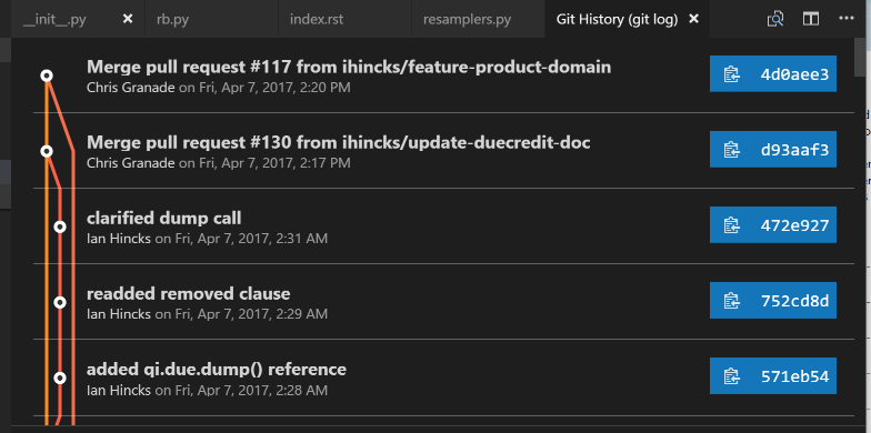
Clicking on any entry in the history visualization presents me with a summary of the changes introduced by that commit, and allows us to quickly make comparisons. This is invaluable in answering that age old question, “what the heck did my collaborators change in the draft this time?”
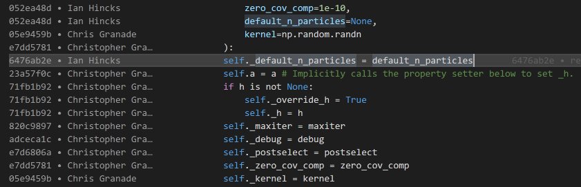
Somewhat related is the GitLens extension, which provides inline annotations about the history of a file while you edit it. By default, these annotations are only visible at the top of a section or other major division in a source file, keeping them unobtrusive during normal editing. If you temporarily want more information, however, press Alt+B to view “blame” information about a file. This will annotate each line with a short description of who edited it last, when they did so, and why.
The last VS Code extension we’ll consider for now is the Project Manager extension, which makes it easy to quickly switch between Git repositories and manage multiple research projects. To use it, we need to do a little bit of configuration first, and tell the extension where to find our projects. Add the following to your user settings, changing paths as appropriate to point to where you keep your research repositories:
"projectManager.git.baseFolders": [
    "C:\\users\\cgranade\\academics\\research",
    "C:\\users\\cgranade\\software-projects"
]
Note that on Windows, you need to use \\ instead of \, since \ is an escape character.
That is, \\ indicates that the next character is special, such that you need two backslashes to type the Windows path separator.
Once configured, press Alt+Shift+P to bring up a list of projects. If you don’t see anything at first, that’s normal; it can take a few moments for Project Manager to discover all of your repositories.
Aside: Viewing TeX Differences as PDFs (Linux and macOS / OS X only)
One very nice advantage of using Git to manage TeX projects is that we can use Git together with the excellent latexdiff tool to make PDFs annotated with changes between different versions of a project.
Sadly, though latexdiff does run on Windows, it’s quite finnicky to use with MiKTeX.
(Personally, I tend to find it easier to use the Linux instructions on Windows Subsystem for Linux, then run latexdiff from within Bash on Ubuntu on Windows.)
In any case, we will need two different programs to get up and running with PDF-rendered diffs. Sadly, both of these are somewhat more specialized than the other tools we’ve looked at, violating the goal that everything we install should also be of generic use. For that reason, and because of the Windows compatability issues noted above, we won’t depend on PDF-rendered diffs anywhere else in this post, and mention it here as a very nice aside.
That said, we will need by latexdiff itself, which compares changes between two different TeX source versions, and rcs-latexdiff, which interfaces between latexdiff and Git.
To install latexdiff on Ubuntu, we can again rely on apt:
$ sudo apt install latexdiff
For macOS / OS X, the easiest way to install latexdiff is to use the package manager of MacTeX.
Either use Tex Live Utiliy, a GUI program distributed with MacTeX or run the following command in a shell
$ sudo tlmgr update --self
$ sudo tlmgr install latexdiff
For rcs-latexdiff, I recommend the fork maintained by Ian Hincks.
We can use the Python-specific package manager pip to automatically download Ian’s Git repository for rcs-latexdiff and run its installer:
$ pip install git+https://github.com/ihincks/rcs-latexdiff.git
Once you have latexdif and rcs-latexdiff installed, we can make very professional PDF renderings by calling rcs-latexdiff on different Git commits.
For instance, if you have a Git tag for version 1 of an arXiv submission, and want to prepare a PDF of differences to send to editors when resubmitting, the following command often works:
$ rcs-latexdiff project_name.tex arXiv_v1 HEAD
Sometimes, you may have to specify options such as --exclude-section-titles due to compatability with the \section command in {revtex4-1} and {quantumarticle}.
arXiv Build Management
Ideally, you’ll upload your reproducible research paper to the arXiv once your project is at a point where you want to share it with the world. Doing so manually is, in a word, painful. In part, this pain originates from that arXiv uses a single automated process to prepare every manuscript submitted, such that arXiv must do something sensible for everyone. This translates in practice to that we need to ensure that our project folder matches the expectations encoded in their TeX processor, AutoTeX. These expectations work well for preparing manuscripts on arXiv, but are not quite what we want when we are writing a paper, so we have to contend with these conventions in uploading.
For instance, arXiv expects a single TeX file at the root directory of the uploaded project, and expects that any ancillary material (source code, small data sets, videos, etc.) are in a subfolder called anc/.
Perhaps most difficult to contend with, though, is that arXiv currently only supports subfolders in a project if that project is uploaded as a ZIP file.
This implies that if we want to upload even once ancillary file, which we certiantly will want to do for a reproducible paper, then we must upload our project as a ZIP file.
Preparing this ZIP file is in principle easy, but if we do so manually, it’s all too easy to make mistakes.
To rectify this and to allow us to use our own project folder layouts, I’ve written a set of commands for PowerShell collectively called PoShTeX to manage building arXiv ZIP archives. From our perspective in writing a reproducible paper, we can rely on PowerShell’s built-in package management tools to automatically find and install PoShTeX if needed, such that our entire arXiv build process reduces to writing a single short manifest file then running it as a PowerShell command.
Let’s look at an example manifest. This particular example comes from an ongoing research project with Sarah Kaiser and Chris Ferrie.
#region Bootstrap PoShTeX
$modules = Get-Module -ListAvailable -Name posh-tex;
if (!$modules) {Install-Module posh-tex -Scope CurrentUser}
if (!($modules | ? {$_.Version -ge "0.1.5"})) {Update-Module posh-tex}
Import-Module posh-tex -Version "0.1.5"
#endregion

Export-ArXivArchive @{
    ProjectName = "sgqt_mixed";
    TeXMain = "notes/sgqt_mixed.tex";
    RenewCommands = @{
        "figurefolder" = ".";
    };
    AdditionalFiles = @{
        # TeX Stuff #
        "notes/revquantum.sty" = "/";
        "figures/*.pdf" = "figures/";
        # "notes/quantumarticle.cls" = $null

        # Theory and Experiment Support #
        "README.md" = "anc/";
        "src/*.py" = "anc/";
        "src/*.yml" = "anc/";

        # Experimental Data #
        "data/*.hdf5" = "anc/";

        # Other Sources #
        # We include this build script itself to provide an example
        # of using PoShTeX in pactice.
        "Export-ArXiv.ps1" = $null;
    };
    Notebooks = @(
        "src/experiment.ipynb",
        "src/theory.ipynb"
    )
}
Breaking it down a bit, the section of the manifest between #region and #endregion is responsible for ensuring PoShTeX is available, and installing it if not.
This is the only “boilerplate” to the manifest, and should be copied literally into new manifest files, with a possible change to the version number "0.1.5" that is marked as required in our example.
The rest is a call to the PoShTeX command Export-ArXivArchive, which produces the actual ZIP given a description of the project.
That description takes the form of a PowerShell hashtable, indicated by @{}.
This is very similar to JavaScript or JSON objects, to Python dicts, etc.
Key/value pairs in a PowerShell hashtable are separated by ;, such that each line of the argument to Export-ArXivArchive specifies a key in the manifest.
These keys are documented more throughly on the PoShTeX documentation site, but let’s run through them a bit now.
First is ProjectName, which is used to determine the name of the final ZIP file.
Next is TeXMain, which specifies the path to the root of the TeX source that should be compiled to make the final arXiv-ready manuscript.
After that is the optional key RenewCommands, which allows us to specify another hashtable whose keys are LaTeX commands that should be changed when uploading to arXiv.
In our case, we use this functionality to change the definition of \figurefolder such that we can reference figures from a TeX file that is in the root of the arXiv-ready archive rather than in tex/, as is in our project layout.
This provides us a great deal of freedom in laying out our project folder, as we need not follow the same conventions in as required by arXiv’s AutoTeX processing.
The next key is AdditionalFiles, which specifies other files that should be included in the arXiv submission.
This is useful for everything from figures and LaTeX class files through to providing ancillary material.
Each key in AdditionalFiles specifies the name of a particular file, or a filename pattern which matches multiple files.
The values associated with each such key specify where those files should be located in the final arXiv-ready archive.
For instance, we’ve used AdditionalFiles to copy anything matching figures/*.pdf into the final archive.
Since arXiv requires that all ancillary files be listed under the anc/ directory, we move things like README.md, the instrument and environment descriptions src/*.yml, and the experimental data in to anc/.
Finally, the Notebooks option specifies any Jupyter Notebooks which should be included with the submission.
Though these notebooks could also be included with the AdditionalFiles key, PoShTeX separates them out to allow passing the optional -RunNotebooks switch.
If this switch is present before the manifest hashtable, then PoShTeX will rerun all notebooks before producing the ZIP file in order to regenerate figures, etc. for consistency.
Once the manifest file is written, it can be called by running it as a PowerShell command:
PS> ./Export-ArXiv.ps1
This will call LaTeX and friends, then produce the desired archive.
Since we specified that the project was named sgqt_mixed with the ProjectName key, PoShTeX will save the archive to sgqt_mixed.zip.
In doing so, PoShTeX will attach your bibliography as a *.bbl file rather than as a BibTeX database (*.bib), since arXiv does not support the *.bib → *.bbl conversion process.
PoShTeX will then check that your manuscript compiles without the biblography database by copying to a temporary folder and running LaTeX there without the aid of BibTeX.
Thus, it’s a good idea to check that the archive contains the files you expect it to by taking a quick look:
PS> ii sgqt_mixed.zip
Here, ii is an alias for Invoke-Item, which launches its argument in the default program for that file type.
In this way, ii is similar to Ubuntu’s xdg-open or macOS / OS X’s open command.
Once you’ve checked through that this is the archive you meant to produce, you can go on and upload it to arXiv to make your amazing and wonderful reproducible project available to the world.
Conclusions and Future Directions
In this post, we detailed a set of software tools for writing and publishing reproducible research papers. Though these tools make it much easier to write papers in a reproducible way, there’s always more that can be done. In that spirit, then, I’ll conclude by pointing to a few things that this stack doesn’t do yet, in the hopes of inspiring further efforts to improve the available tools for reproducible research.
- Template generation: It’s a bit of a manual pain to set up a new project folder. Tools like Yeoman or Cookiecutter help with this by allowing the development of interactive code generators. A “reproducible arXiv paper” generator could go a long way towards improving practicality.
- Automatic Inclusion of CTAN Dependencies:
Currently, setting up a project directory includes the step of copying TeX dependencies into the project folder.
Ideally, this could be done automatically by PoShTeX based on a specification of which dependencies need to be downloaded, a la pip’s use of
requirements.txt. - arXiv Compatability Checking:
Since arXiv stores each submission internally as a
.tar.gzarchive, which is inefficient for archives that themselves contain archives, arXiv recursively unpacks submissions. This in turn means that files based on the ZIP format, such as NumPy’s*.npzdata storage format, are not supported by arXiv and should not be uploaded. Adding functionality to PoShTeX to check for this condition could be useful in preventing common problems.
In the meantime, even in lieu of these features, I hope that this description is a useful resource. ♥
Acknowledgements
- A huge thanks to Daniel Suess for writing the install instructions on macOS / OS X! ★♥★
- Thanks to Olivia Guest for suggestions on Git tutorials.
- Thanks to Ben Barigola, Sarah Kaiser, and Chris Ferrie for feedback on drafts and for help testing.
- Thanks to Chris Ferrie for nerdsniping me into writing this post.