Assessing and Controlling Quantum Information Processing Devices
Cassandra E. Granade
Centre for Engineered Quantum Systems
$
\newcommand{\ee}{\mathrm{e}}
\newcommand{\ii}{\mathrm{i}}
\newcommand{\id}{𝟙}
\newcommand{\TT}{\mathrm{T}}
\newcommand{\defeq}{\mathrel{:=}}
\newcommand{\Tr}{\operatorname{Tr}}
\newcommand{\expect}{\mathbb{E}}
\newcommand{\sbraket}[1]{\langle\!\langle#1\rangle\!\rangle}
$
This talk can be summarized in one slide.
\begin{equation} \Pr(\text{model} | \text{data}) = \frac{\Pr(\text{data} | \text{model})}{\Pr(\text{data})} \Pr(\text{model}) \end{equation}
OK, Two Slides
Bayesian methods for experimental data processing work.
More Seriously
How do we assess if quantum computing is possible, given an experimental demonstration of a prototype?
We don't.
(Classical computing is impossible.)
What Do We Mean Classically?
Colloquially, a classical computer is something that acts in most ways and for most of the time like we would expect a classical computer to act.
Classical computing models preclude some error sources (comets, the NSA, etc.).
Take-away for quantum applications: we need to make and state assumptions, and to qualify our conclusions.
To a Bayesian, this means we need to be careful to record our priors.
(Frequentism uses priors, too: they're called models.)
What models and priors should we use to evaluate QIPs?
State Model, or a Little Thing Called Tomography
Born's rule gives predictions in terms of a state $\rho$, \[ \Pr(E | \rho) = \Tr[E \rho] \] for a measurement effect $E$.
This is a likelihood, so use Bayes' rule to find the state $\rho$. [Jones 1991, Blume-Kohout 2010]
Numerical evaluation is a kind of classical simulation.
Numerical Algorithm
We use sequential Monte Carlo (SMC) to compute Bayes updates.
\begin{align} \Pr(\rho) & \approx \sum_{p\in\text{particles}} w_p \delta(\rho - \rho_p) \\ w_p & \mapsto w_p \times \Pr(E | \rho_p) \end{align}
Uses simulation as resource.
Gives estimates of posterior over states $\rho$. Lots of advantages:
- Region estimation [Ferrie 2014]
- Model selection and averaging
[Wiebe et al 2014, Ferrie 2014] - Hyperparameterization [Granade et al 2012]
Easy to Implement
import qinfer as qi
basis = qi.tomography.gell_mann_basis(3)
prior = qi.tomography.GinibreDistribution(basis)
model = qi.BinomialModel(qi.tomography.TomographyModel(basis))
updater = qi.smc.SMCUpdater(model, 2000, prior)
heuristic = qi.tomography.rand_basis_heuristic(updater, other_fields={
    'n_meas': 40
})
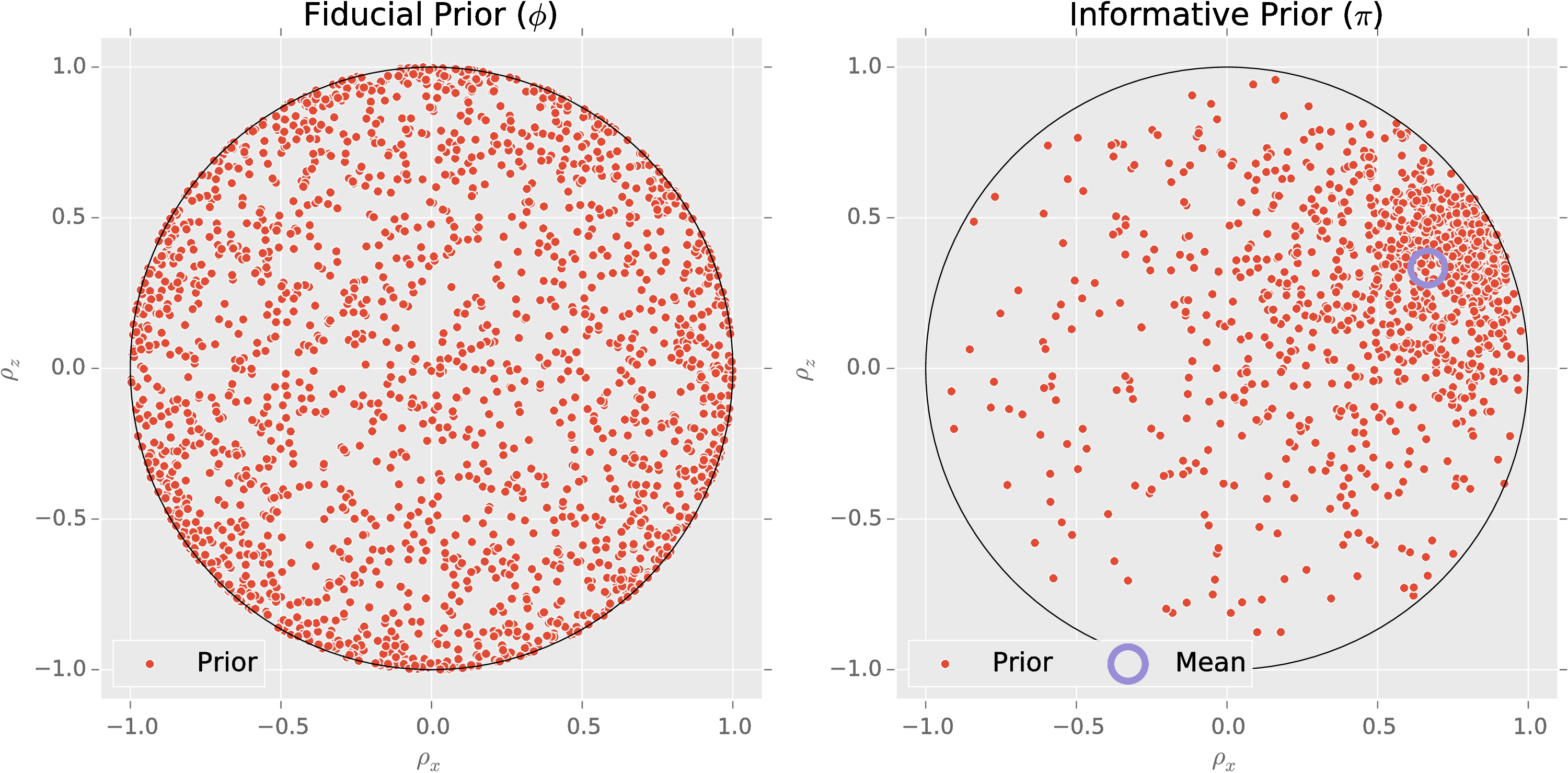
Informative Priors
How do we encode the assumption that the state $\rho$ is near a state $\rho_\mu$?
We use amplitude damping to contract uniform prior $\pi(\rho)$ [Granade and Combes (upcoming)].
Choose $\rho_*$, $\alpha$, $\beta$ such that $\expect[\rho_{\text{sample}}] = \rho_\mu$ and $\expect[\epsilon]$ is minimized.
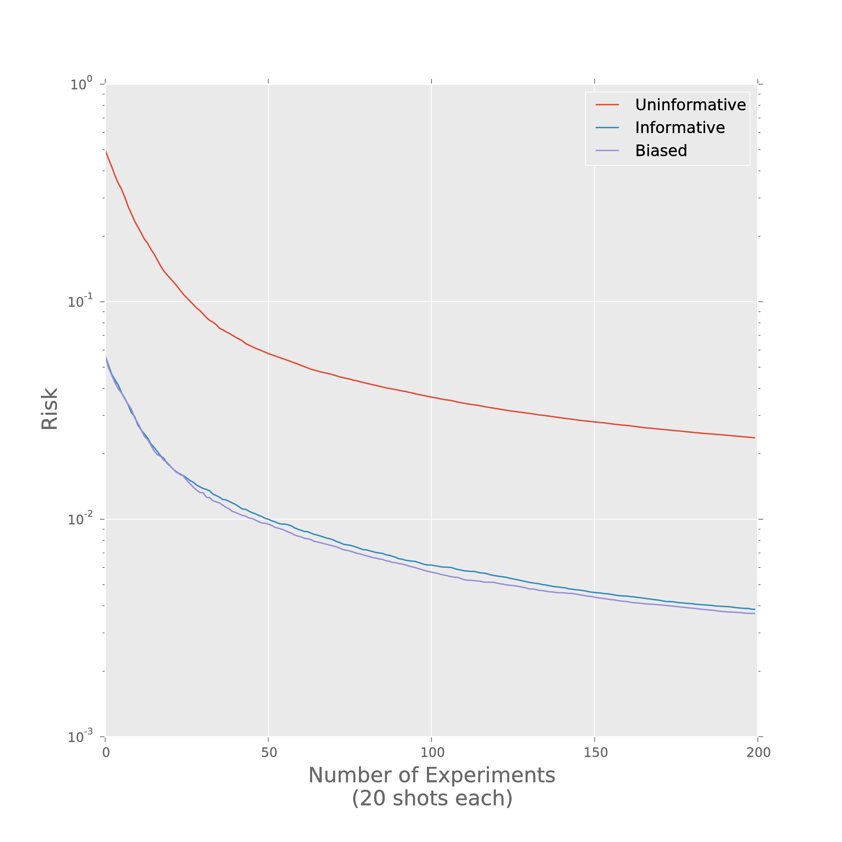
Prior Information Really Helps
Posterior covariance characterizes uncertainty.
Example: depolarizing channel dominates uncertainty in our QPT simulation.
State-Space State Tomography
(Useful in space.)
We don't need to assume that the "true" state follows a random walk.
Can also consider other models.
Hamiltonian Evolution (aka Frequency Estimation)
\[ U(t) = \ee^{-\ii H t} \]
Does the device evolve under the correct $H$? Does a simulator implement the correct $H$?
As before, we can answer this using simulation as a resource.
- Classical resources (particle filters, rejection sampling).
[Granade et al 2012] - Quantum resources (semiquantum particle filters).
[Wiebe et al 2014] - Small quantum resources (quantum bootstrapping).
[Wiebe et al 2015]
The prior $\pi(H)$ again encodes the assumptions that we make about $H$.
Examples
\begin{align} H(\vec{x}) & = \sum_{\langle i, j \rangle} x_{i,j}\,\sigma_z^{(i)} \sigma_z^{(j)} \\ H(\vec{x}) & = \sum_{i,j,\alpha,\beta} x_{i,j,\alpha,\beta}\,\sigma_{\alpha}^{(i)} \sigma_{\beta}^{(j)} \end{align} Can also include Hermitian generators as well as skew-Hermitian. \begin{align} L(\omega, T_2) & = -\ii \omega (\id \otimes \sigma_z - \sigma_z^\TT \otimes \id) + \frac{1}{T_2} \left( \sigma_z^\TT \otimes \sigma_z - \id \otimes \id \right) \end{align}
Model selection provides a way to test assumptions by progressively considering more general models.
AIC, ABIC, Bayes factor, model-averaged estimation, etc.
\begin{align} \text{BF}(A : B) & \defeq \frac{\Pr(A | \text{data})}{\Pr(B | \text{data})} = \frac{\Pr(\text{data} | A) \Pr(A)}{\Pr(\text{data} | B) \Pr(B)} \end{align}
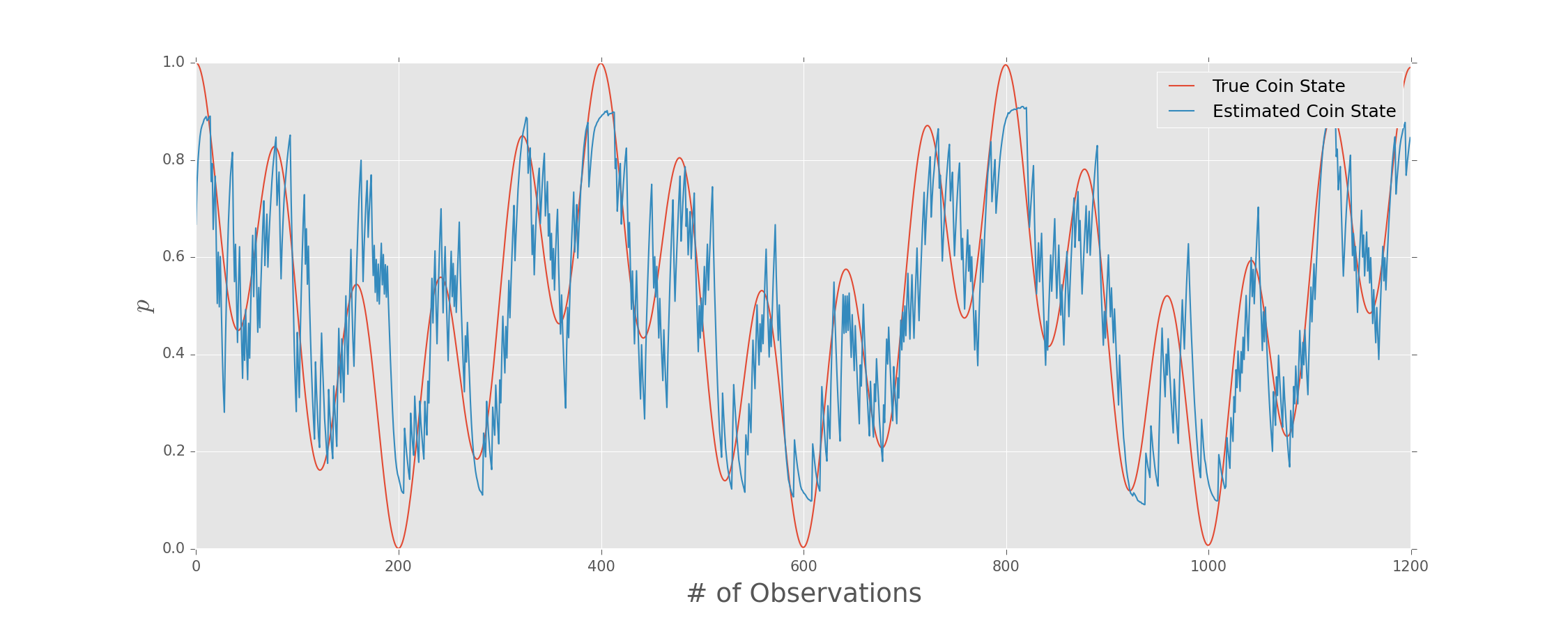
Example: Detecting Drifting Parameters
\[ \Pr(\text{O-beam} | A, b, \phi; \theta) = \frac{1 + b}{2} + \frac{A}{2} \cos(\phi + \theta) \]
Compare models $\phi \ne \phi(t)$ and $\phi$ following a Markovian Gaussian process.
We analyze the same data with both models, recording the total likelihood as we go.
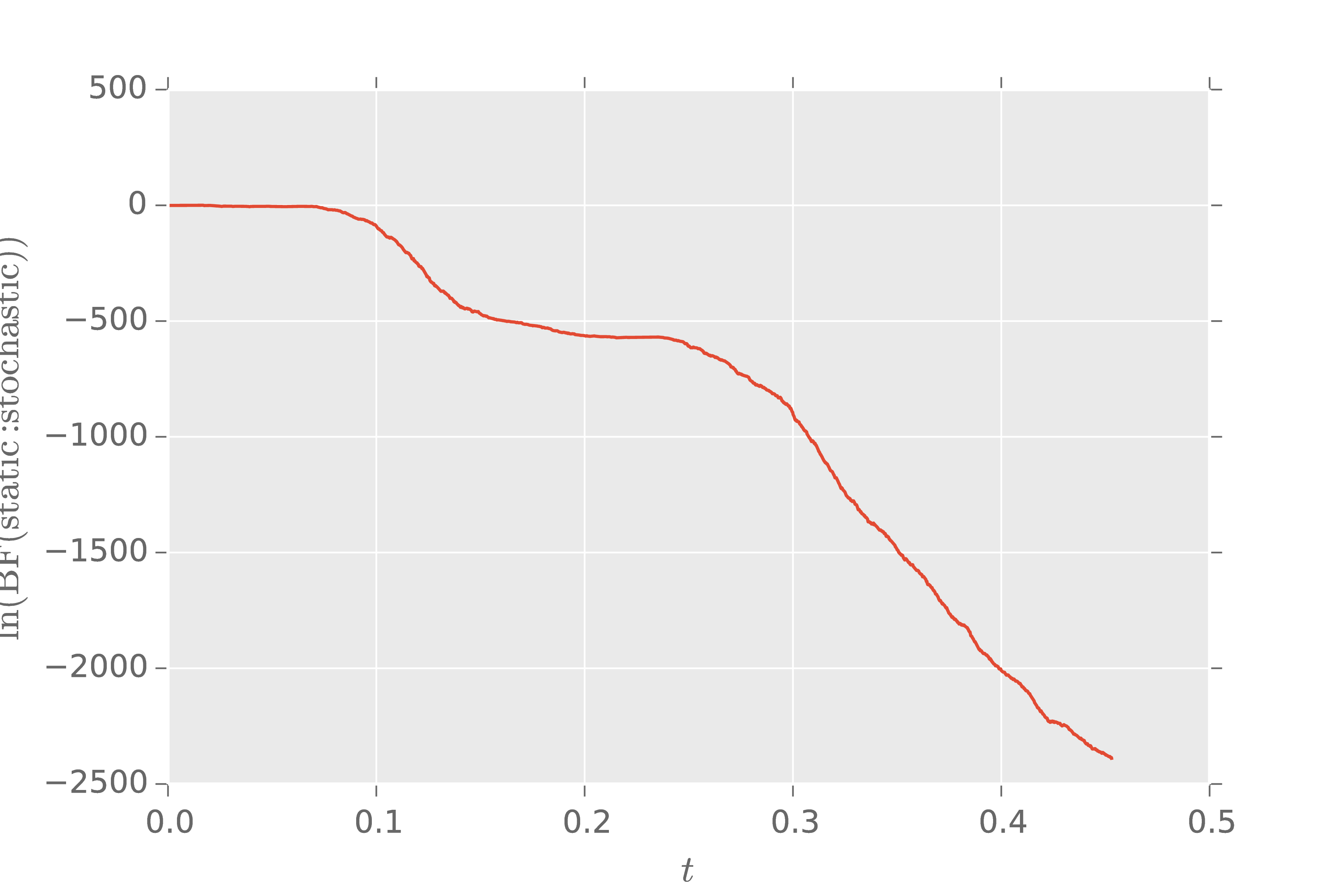
Using Bayes factor analysis, we can conclude that the drifting model better explains the observed data.
Using Bayesian inference, Hamiltonian learning can proceed adaptively.
Necessary [Hall and Wiseman 2012] and sufficient [Ferrie et al 2013] for exponential improvement in the number of experiments required to learn Hamiltonians.
For building algorithms, more convenient to use circuits than continuous-time evolution.
Gate Model
Can enforce the gate model to some degree with how we design our pulses. We can use more general simulation methods (e.g.: cumulant [Cappellaro et al 2006]) to reason about validity of the gate model.
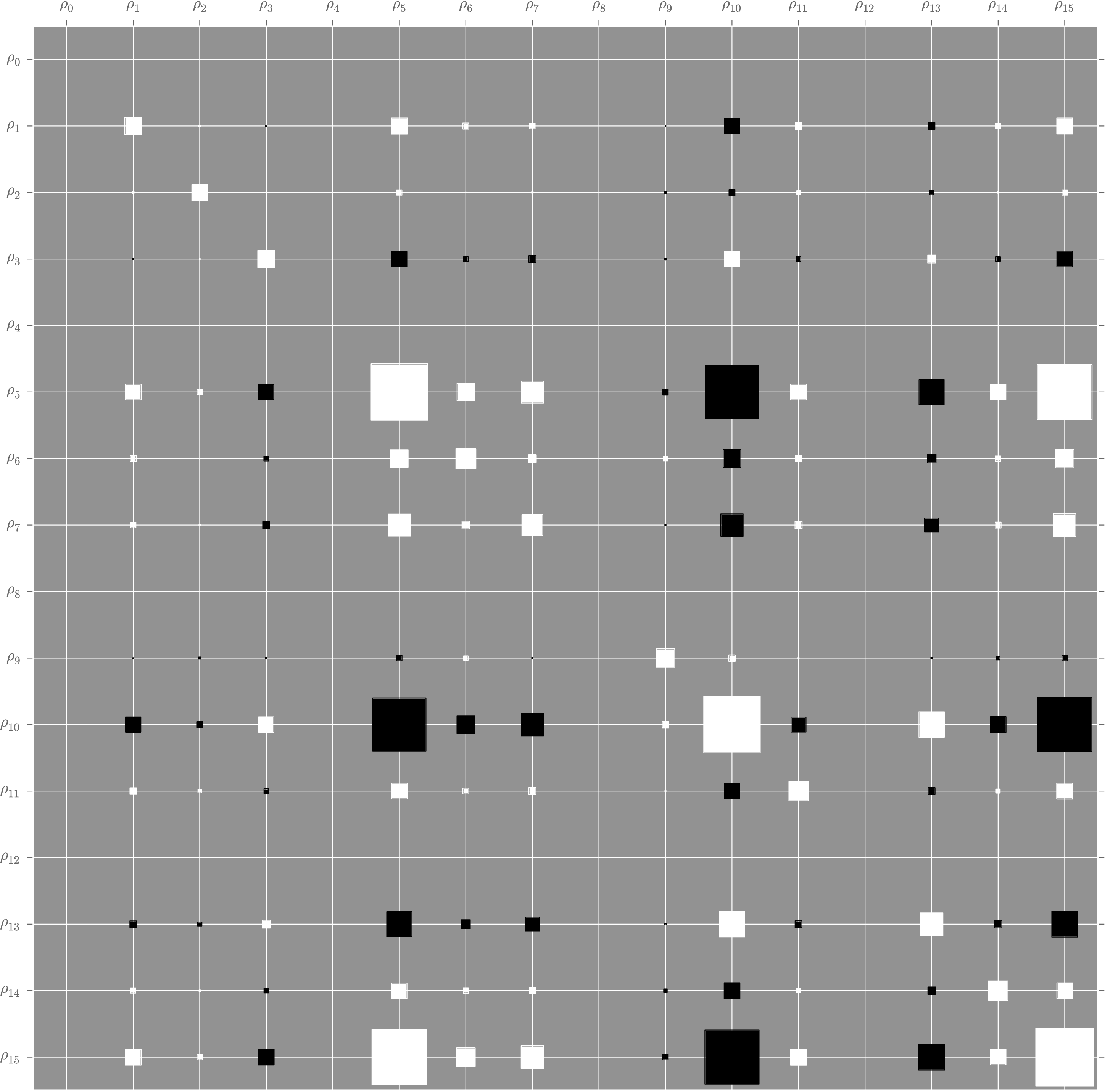
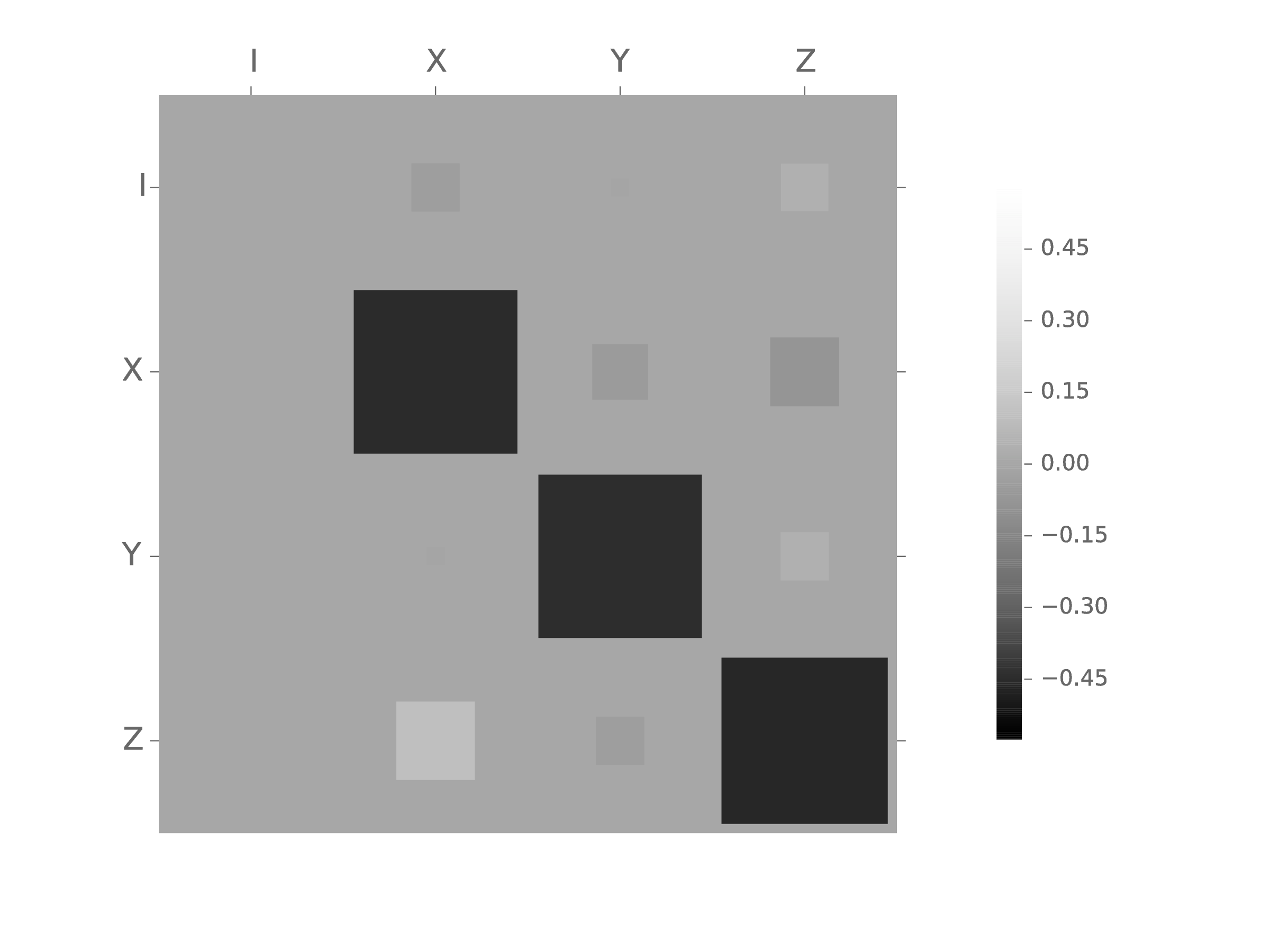
Process Tomography
Same techniques as before apply to enable learning snapshots of dynamics. Choi-Jamiołkowski isomorphism lets us rewrite process tomography as (ancilla-assisted) state tomography.
\[ \Tr[E \Lambda(\rho)] = \Tr[(\id \otimes E) J(\Lambda) (\rho^\TT \otimes \id)] = \sbraket{\rho^\TT, E | J(\Lambda)} \]
This is difficult: limited to sampling statistics, no exponential improvement from longer evolutions.
Want something more like Hamiltonian learning. Recent example: gate set tomography [Blume-Kohout et al 2013]. GST is in turn difficult due to parameter count.
What do we actually want out of our gate model?
The Gate Model and Fidelity
Common to describe gate models in terms of the average gate fidelity. If errors are not strongly gate-dependent, also common to quote AGF averaged over gates.
For some models, AGF can describe error correcting thresholds. More generally, unreasonably strong assumptions may be needed [Sanders et al 2015].
All the same, let's keep searching under the streetlight, keeping track of our assumptions.
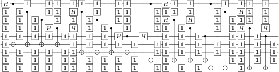
Randomized Benchmarking for Fun and Profit
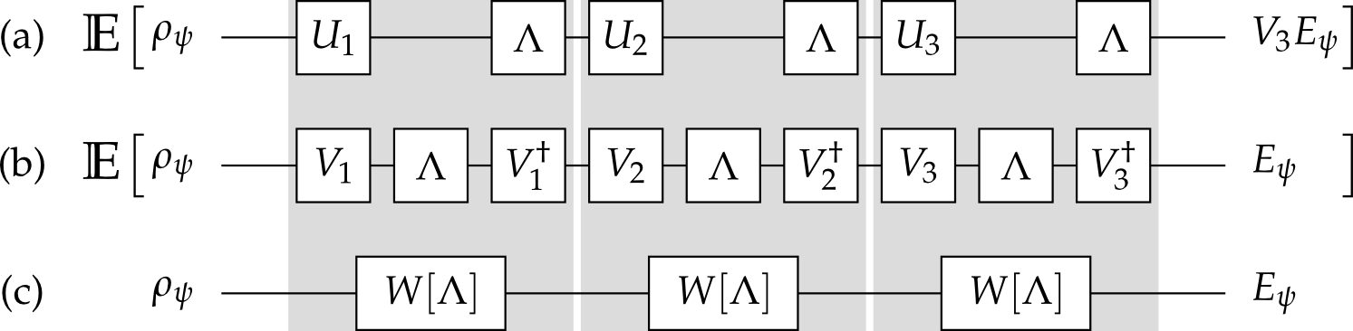
By choosing random sequences $\{U_1, U_2, \dots\}$, can implement twirling superchannel $W[\cdot]$ with imperfect gates.
Marginalization and Simulation Costs
Marginalizing over sequence choice removes quantum simulation, yielding simple (scalar!) algebraic models.
\begin{align} \Pr(\text{survival} | A, B, p; m) & = A p^m + B \\ A & \defeq \Tr(E \Lambda[\rho - \id / d]) \\ B & \defeq \Tr(E \Lambda[\id / d]) \\ p & \defeq \frac{dF - 1}{d - 1} \end{align}
We now have a simulation-free likelihood function that assesses average gate fidelity.
This is ideal for embedded applications.
Embedded Bayesian Inference
Rejection sampling with Gaussian resampling allows for constant-memory embedded Bayesian inference [Wiebe and Granade (upcoming)].
Less general than SMC, but significantly faster and more parallelizable. Ideal for FPGA-based estimation of randomized benchmarking model.
Modern experiment control via FPGAs, so embed inference directly in control hardware to make an online fidelity oracle.
Accelerated Randomized Benchmarking
We have lots of prior information: each pulse is a pertubation of a pulse we've already characterized.
Since we're being honest frequentists (aka Bayesians), let's use that to accelerate estimation.
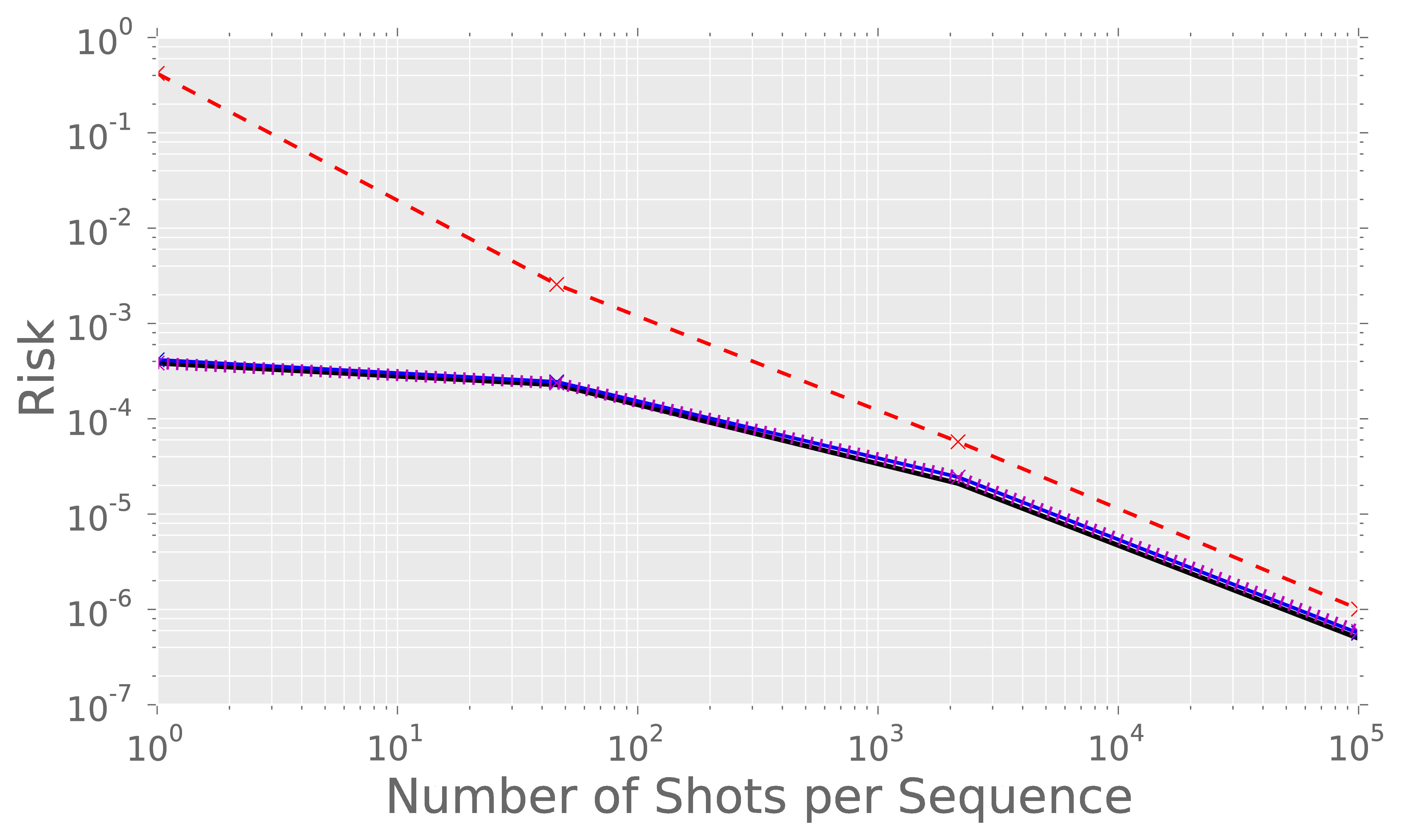
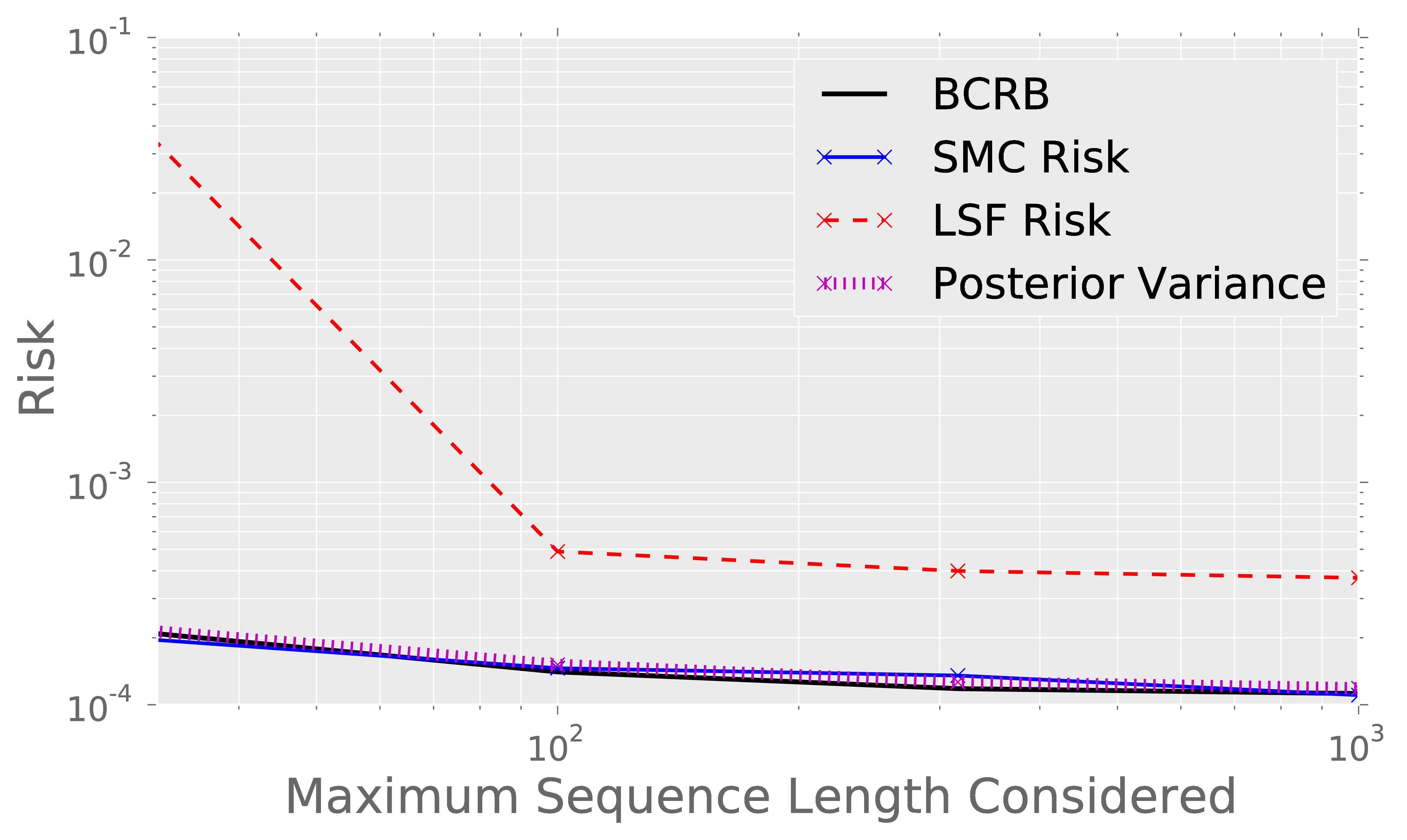
With lots of data, least-squares fitting works fine, but it isn't stable with small amounts of data. Bayesian inference is nearly optimal for the strong prior.
Only remaining simulation cost: reduction of pulses to gates.
...but nature does this for us.
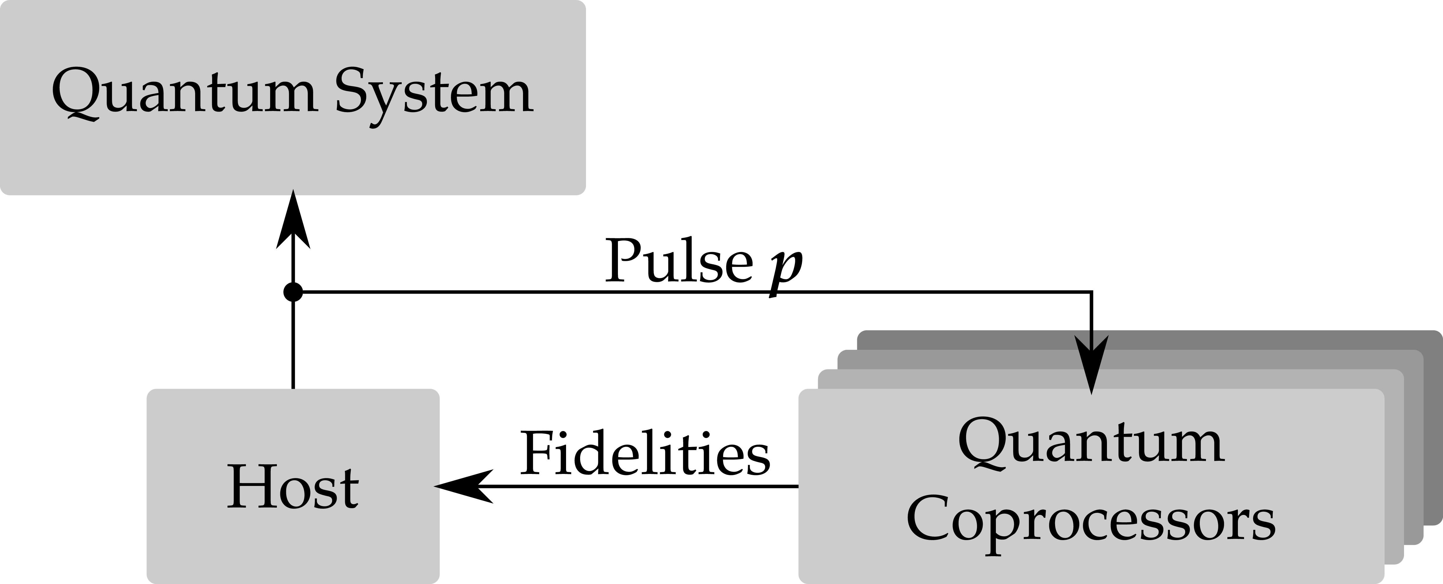
Use array of quantum coprocessors to evaluate pulses in parallel, for different hypotheses about the true evolution. [Granade 2015]
Flip the Problem Around
How do we make a useful quantum device?
Treat characterization parameters as fitness functions.
Pulse Design
Optimal control using AGF $F$ as a fitness has been applied very successfully to design pulses.
Khaneja derivative allows for using gradient-ascent methods to optimize $F$.
Other Fitness Functions
- Leakage
- Unitarity
- Haas-Puzzuoli decoupling fitness
Several of these fitness functions can also be experimentally measured using randomized benchmarking.
- $F$: interleaved 2-design twirl
- Leakage: 1-design twirl
- Unitarity: 2-design twirl on two copies
Using the same techniques, then, we can embed fidelity, leakage and unitarity estimation all into control hardware.
Immediately allows embedding RB-based pulse optimization.
- Ad-HOC / ORBIT [Egger and Wilhelm et al 2014, Kelly et al 2014]
- ACRONYM [Ferrie and Moussa 2014]
MOQCA
Multi-objective genetic algorithms can be used to design pulses that work over a range of models.
- Memetic step
- ACRONYM / SPSA
- Evolutionary Strategies
- Mutation rate, memetic paramteters co-evolve
- Tournaments
- Randomly selected from ensemble of tournament fns.
MOQCA is black-box for its oracle. Robust against noisy oracles.
Not the most efficient, but could possibly work in much larger systems and with other kinds of distortions.
Example: $\left.\frac{\pi}{2}\right)_x$
We consider controls up to $70$ MHz, but we want robustness to $\pm 100$ kHz static field, ringdown distortion, imperfect measurement of distortion.
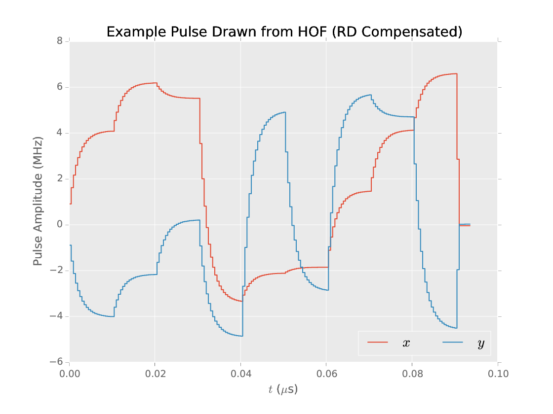
Memetic optimization finds Pareto optimal pulses with fidelity $\ge 0.99$.
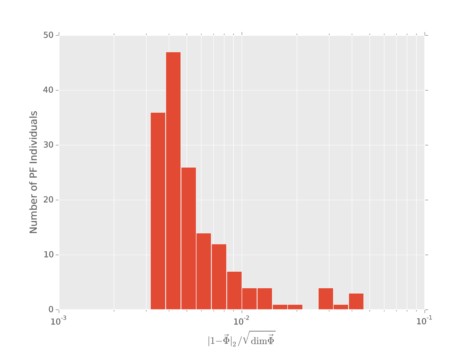
200 generations, 140 individuals, 5 hypotheses ($\pm 100 \text{kHz}$), noisy evaluation of distortion (~20 dB SNR)